With the rapid growth of data and computing resources, Machine Learning (ML) technology is playing an increasingly important role in more and more areas. For some physical phenomena expressed by partial differential equations, it is difficult for traditional methods to solve complex situations such as high dimensions. Universal approximation theorem^[1] enables deep neural networks (DNNs) to solve variational function problems. The deep learning based method proposed in this paper is a new solution, by minimizing the difference between variational functions and partial differential equations, DNN can transform physical problems^[2] into optimization problems^[3] that can be solved with modern deep learning libraries.

In the case of variational equations, physical constraints play an essential role^[4–8]. In this paper, instead of using DNN to represent the wave function directly, we use DNN to represent the cumulative distribution function (CDF) $ \int_{-\infty}^{x} f(x') {\mathrm{d}}x' $ of the wave function $ \psi(x) $. In order to improve the efficiency of data learning, we apply the unitary constraint to the variational function, and the whole computational process does not need to compute numerical integration, thus greatly reducing the computational amount. These advantages make the method in this paper more suitable for dealing with multiple problems with a large amount of computation.

In this paper, we reviewed that physically constrained neural networks can be used as efficient trial wave functions in solving Schrodinger equations with the harmonic oscillator and the Woods-Saxon potential. We have also extended this method to Schrodinger equation with the double-well potentials in the same framework.

Unlike the previous direct expression of the wave function by the Variational Artificial Neural Networks (VANN)^{[5, 9–11]}, we obtain the wave function indirectly through the CDF, and the relationship between the two is as follows

where $ F(x) $ is the CDF, $ \psi(x) $ is the wave function. Auto differentiation (auto-diff)^[12] tools in deep learning libraries can be used to compute the derivative $ {\mathrm{d}}F/{\mathrm{d}}x $. The wave function obtained by the CDF satisfies the normalisation, thus avoiding numerical integration and simplifying the calculation. Furthermore, the value range of the CDF is between (0, 1), which makes it much easier to train. Due to the above two advantages, our algorithm has less computation and training cycles, while maintaining good accuracy.

The input of the neural network is the n-dimensional spatial coordinates x. The first layer of the DNN has $ m=32 $ hidden neurons whose values are computed by $ h_1 = \sigma(x W_1 + b_1) $, where $ W_1 $ is the weight matrix with $ n\times m $ elements and $ b_1 $ is the bias vector with m values. To avoid linear superposition, a non-linear function σ, called the activation function, is introduced, which can improve the representational ability of the DNN. The second layer works similarly, taking the output of the first layer as the input of the second layer $ h_2 = \sigma(h_1 W_2 + b_2) $, allowing multiple hidden layers to be stacked. The last layer returns the value of the CDF.

Since the CDF is monotonic, the variational function of the DNN fitting must also be monotonic. To solve this problem, we add a non-negative constraint to the weight $ W_i $. Theoretically, nonlinear functions such as sigmoid, tanh and relu can all be used as the activation function of the DNN, but in practice, since we need continuous and monotonic activation functions, and the derivative cannot be 0, we finally choose the sigmoid function as the activation function, which satisfies the above conditions. And the sigmoid function has a range of (0, 1), which guarantees the output range of the last layer.

The goal of the training is to minimise the violation between the wave function obtained by the DNN and the Schrodinger equation, so that the ground state energy and the corresponding wave function can be found,

where $ H = -{\hbar^2 \over 2m} \nabla^2 + V({\bf x}) $ is the Hamiltonian operator and $ E_0 $ represents its smallest eigenvalue. The loss function is defined as follow,

where θ is a trainable parameter, including $ W_i $, $ b_i $ and $ E_0 $, $ E_0 $ is another trainable parameter initialised to 0. DNN guarantees that ψ satisfies the Schrodinger equation by minimising the first term, and the other two terms guarantee that the CDF fitted by DNN satisfies the boundary conditions. The range of the CDF provides normalisation of the wave function, which simplifies the calculation.

Note that the initial values of the trainable parameters $ W_i $ and $ b_i $ are usually initialised randomly or in the Xavier scheme^[13]. In our work, however, the initialisation scheme of the parameter has little effect on the result, so we use random initialisation.

We add another loss term $ {\rm e}^{\gamma E_0} $, where γ is a small value. By subtracting this term from the loss function, integration is avoided and DNN optimizes the loss function to make $ E_0 $ lower. By training this energy term, the ground state energy and the ground state wave function can be obtained with small error^[14].

We tested the performance of the DNN Schrodinger equation solver on three classical quantum mechanical problems. The first problem is the harmonic oscillator model^[15], the potential of the harmonic oscillator can be written as,

where m is the mass of the oscillator, ω is its angular frequency and x is its deviation from equilibrium position.

The second example is to solve Schrodinger equation with Woods-Saxon potential^[16],

where $ a_0 $ is the thickness of the surface layer and the average radius is given as $ R_0 $.

The third is a double-well potential problem, which is a new potential added to our previous work^[14]. The potential in the Hamiltonian can be written as:

Where h, l, a respectively control the depth, position, and width of the double-well. Unlike the previous questions,the ground state wave function of a double-well potential problem will exhibit two peaks. Applying our method to such a potential can further verify the universality of the architecture.

For simplicity, some parameters are set as follows,

The input to DNN is an unordered list of domain coordinates. The ground state energy and the CDF are obtained by minimising the terms of the loss function, and thus the ground state wave function is obtained indirectly. Unlike the previous method of solving the Schrodinger equation using supervised learning, our method belongs to unsupervised learning. The wave function is usually very close to the exact wave function after training the DNN through iterations in harmonic oscillator, Woods-Saxon potential, infinitely high potential well^[14] and a double-well potential. DNN can get very accurate results after 2 000 iterations, but we trained 10 000 times, using a very small learning rate in the last 1 000 times.

We used Adam algorithm^{[14, 17–18]} that add momentum mechanism and adaptive learning rate to the simple stochastic gradient descent,

where θ represents the model parameters, including weights and biases within a neural network, The term n denotes the current iteration number, reflecting the step in the iterative process of optimization. ‘lr’, the learning rate, is a critical hyperparameter that controls the size of the steps taken towards the minimum of the loss function. m is the batch size, which determines the number of samples used for each parameter update. $ {\partial l_i \over \partial \theta} $ represents the gradient of the loss function $ l_i $ with respect to θ, guiding the direction and magnitude of parameter adjustments.

We use a learning rate scheduler to speed up the training, setting a higher learning rate in the early stages to speed up convergence, and a lower learning rate in the later stages to reach the global minimum.

To quantify the difference between the wave function obtained by DNN $ \psi_{\rm DNN} $ and the real wave function $ \psi_{\rm true} $, we introduce the partial wave fidelity K,

The closer the K is to one, the closer the result of DNN is to the exact wave function.

For the harmonic oscillator problem, DNN can control the ground state energy error within 0.06% after 1 500 training, and reduce the error to 0.002% after 10 000 training, the partial wave fidelity K is 0.999 996 7 when using 4 hidden layers with 16 units per layer. To study the influence of the number of variational parameters on the training results, K is discussed in Ref. [14] by using different numbers of hidden layers and units per layer.

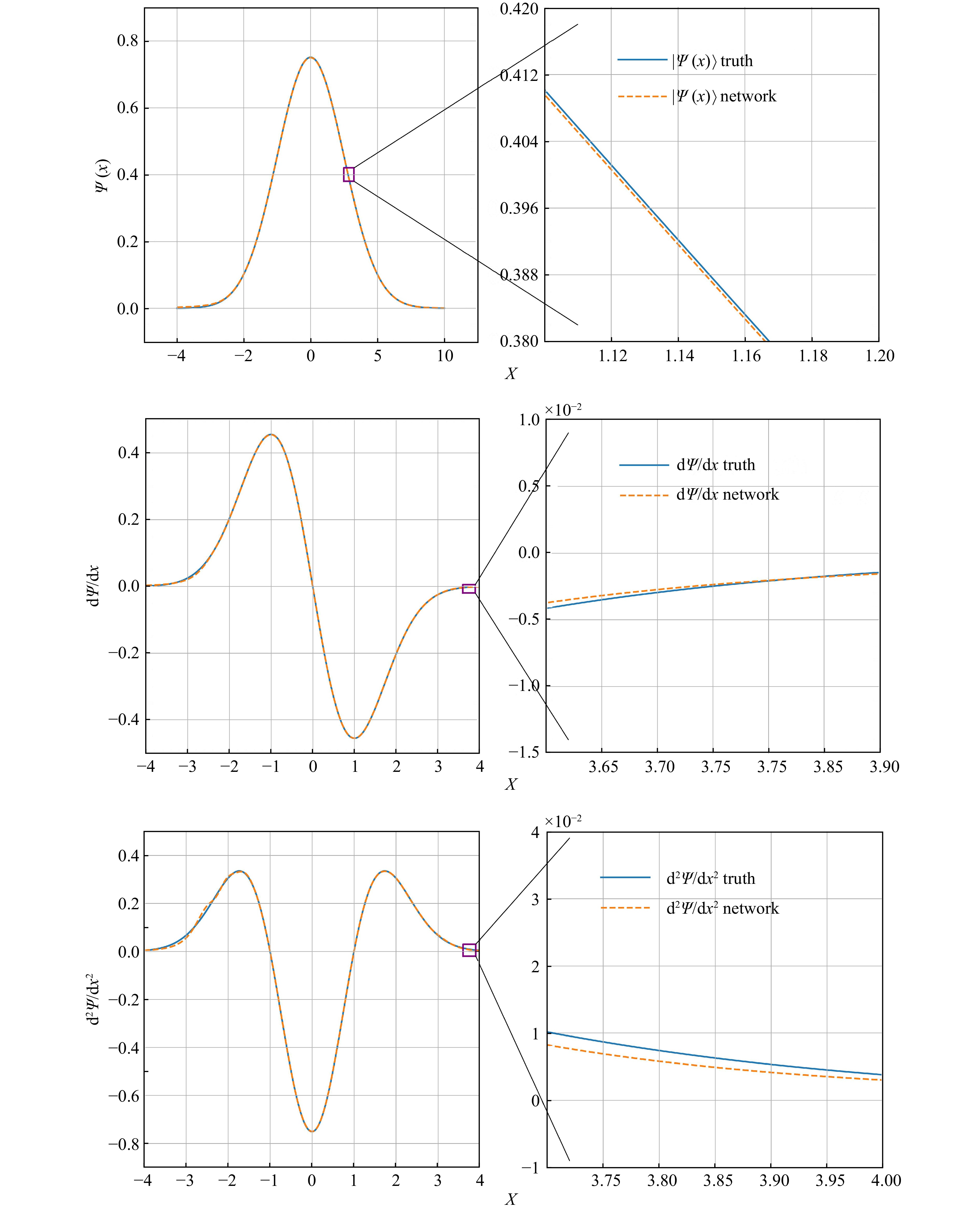
To understand the difference between the wave function obtained by DNN and the real wave function, we calculate the CDF, the wave function and the first and second derivatives of the wave function respectively.

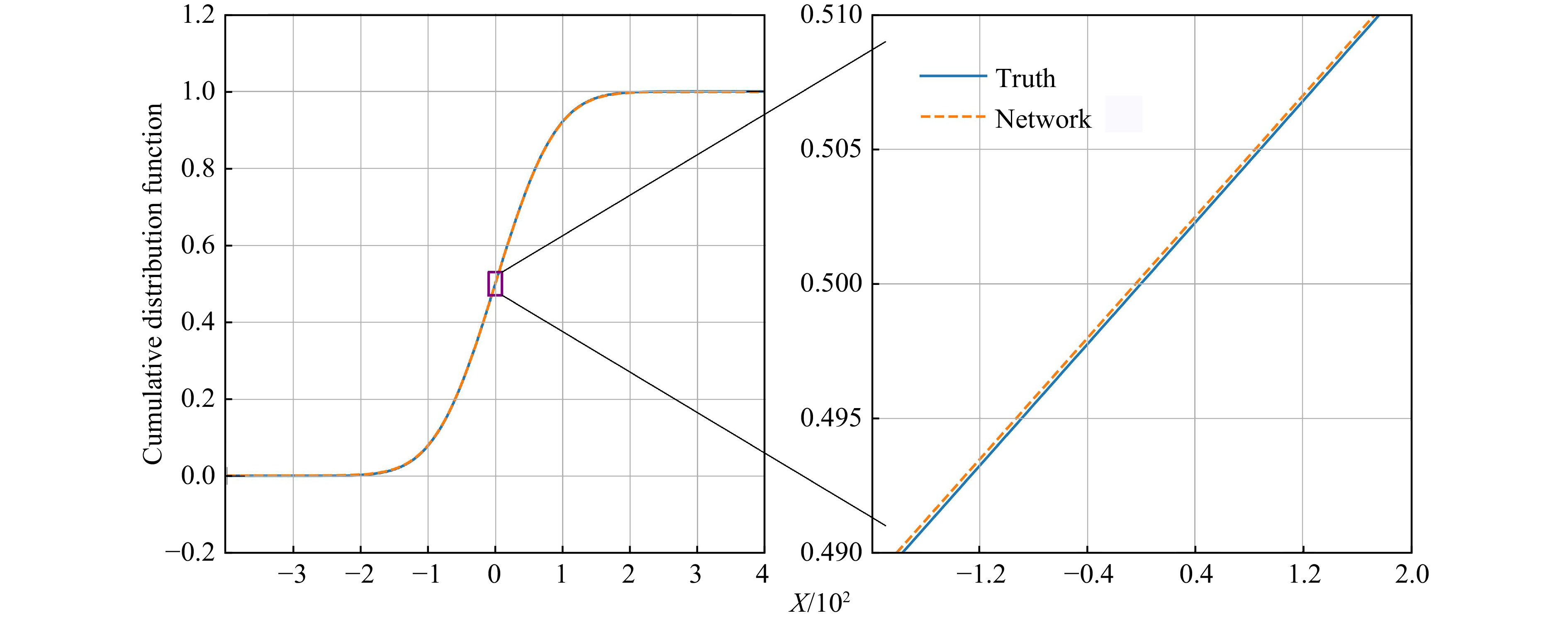
The error between the CDF fitted by DNN and the real CDF is within 0.000 1 as shown in Fig. 1. The error range of the ground state wave function can be controlled within 0.000 2 as shown in Fig. 2. In addition, the accuracy of the first and second derivatives of the wave function obtained by the DNN is also very high, which means that the DNN has learned the real physical information of the wave function.

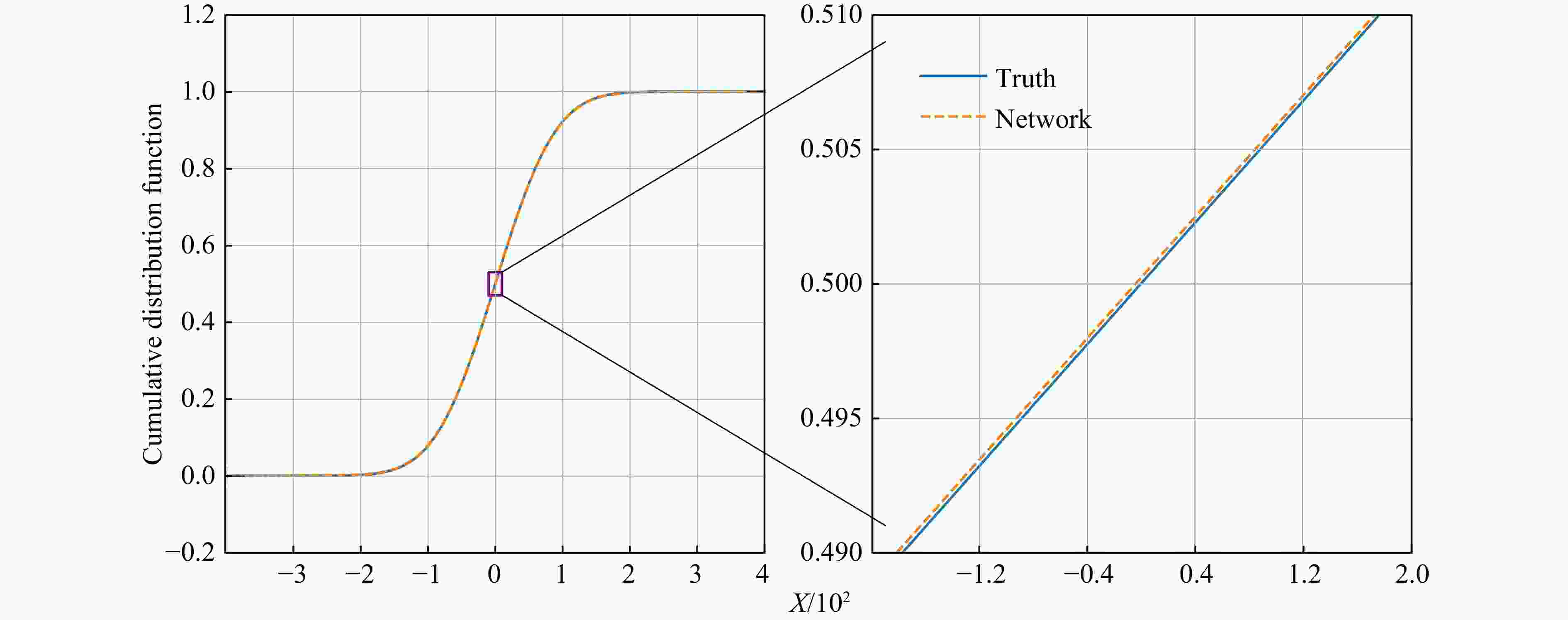
Figure 1.  One-dimensional harmonic oscillator’s CDF^[14]

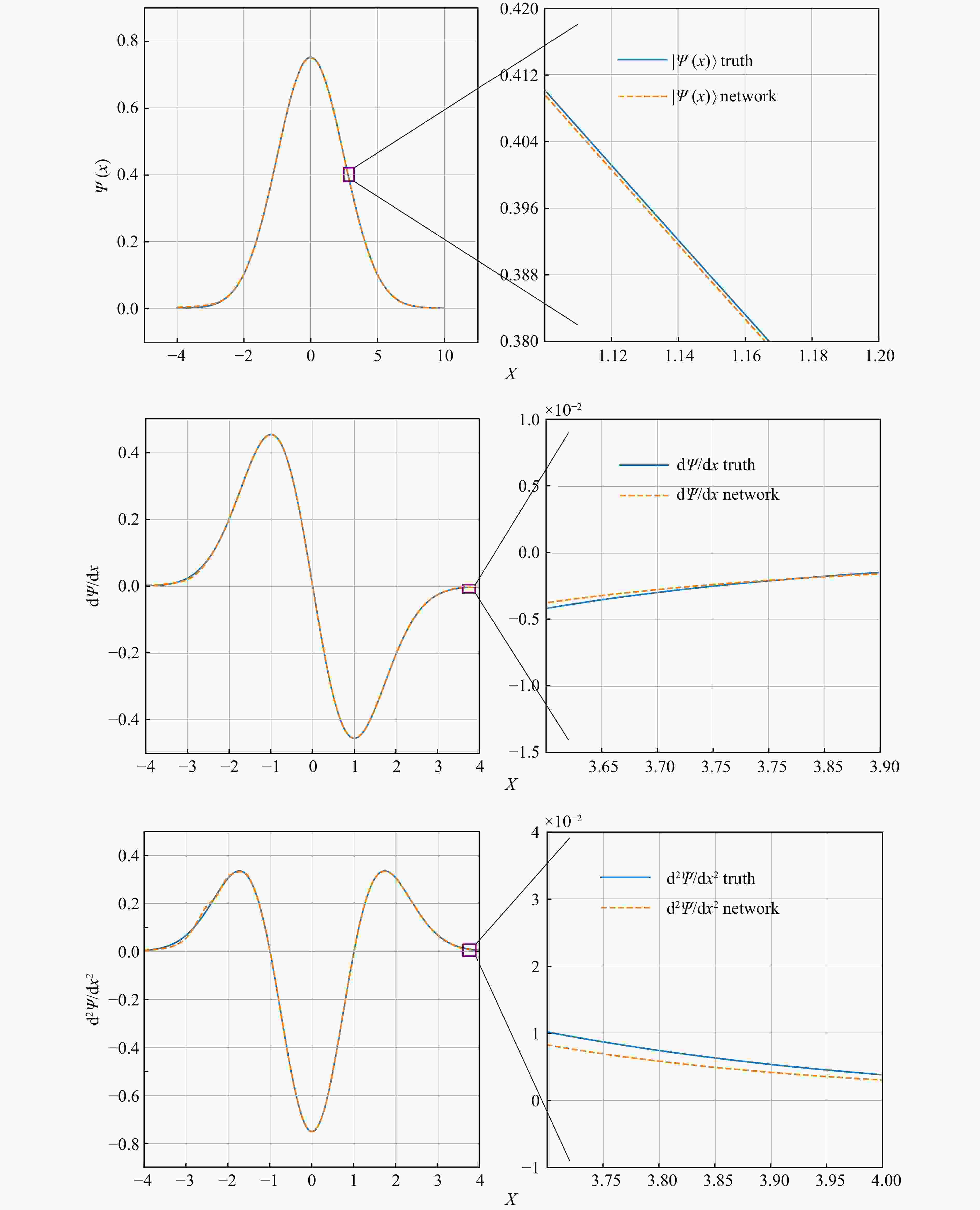
Figure 2.  One-dimensional harmonic oscillator's ground state wave function(top panel), and it’s first derivative(central) and the second derivative(bottom)^[14].

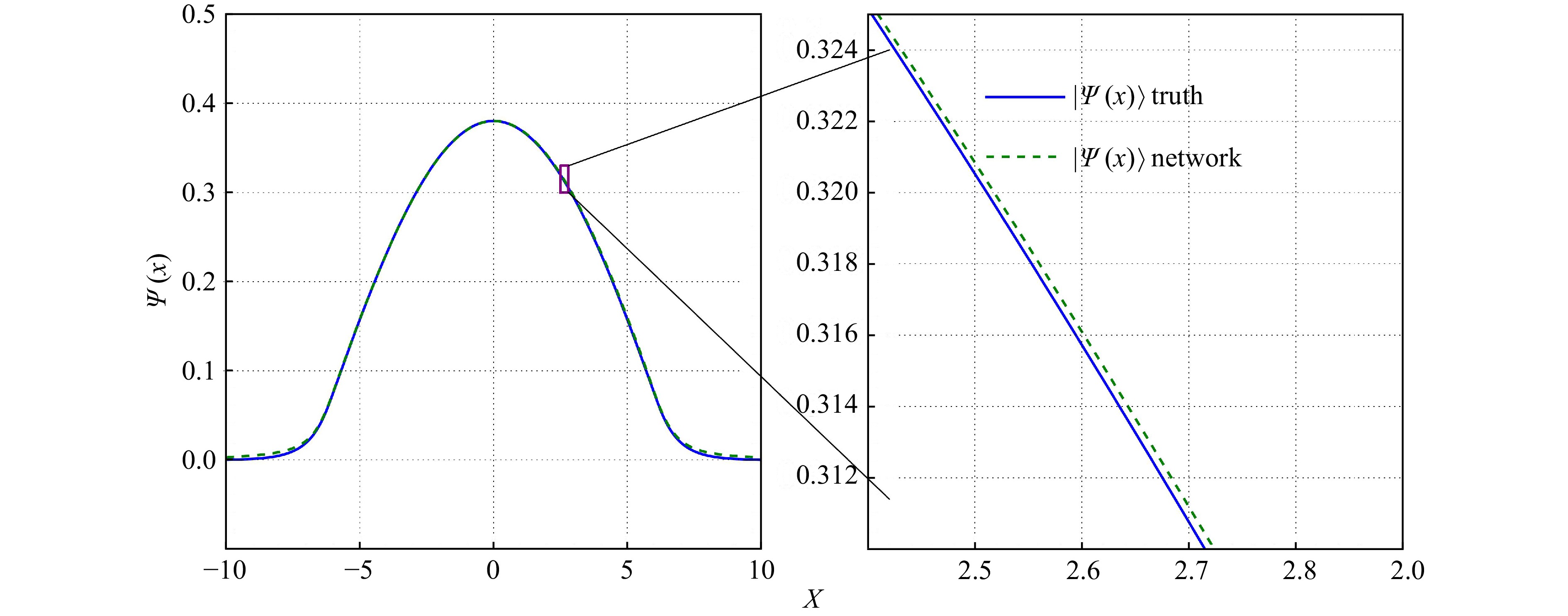
We verified the universality of the method by using the same network to solve the Schrodinger equation with the Woods-Saxon potential and the double-well potential. For the Schrodinger equation with Woods-Saxon potential energy, using the same parameter γ in the harmonic oscillator potential, the Woods-Saxon potential could control the error of the ground state energy less than 0.02%. Fig. 3 shows the comparisons between the learned ground state wave function and the true values. It can be seen that the ground state wave function obtained from the DNN also agrees very well with the exact solution. The error range can be controlled within 0.000 2 for the ground state wave function of the Woods-Saxon potential as shown in Fig. 3. And the ground state energy calculated by the DNN for the Woods-Saxon potential problem is −0.973 82, which is also within an error of 0.002% to the exact result of −0.973 85 and $K=0.999\,964$.

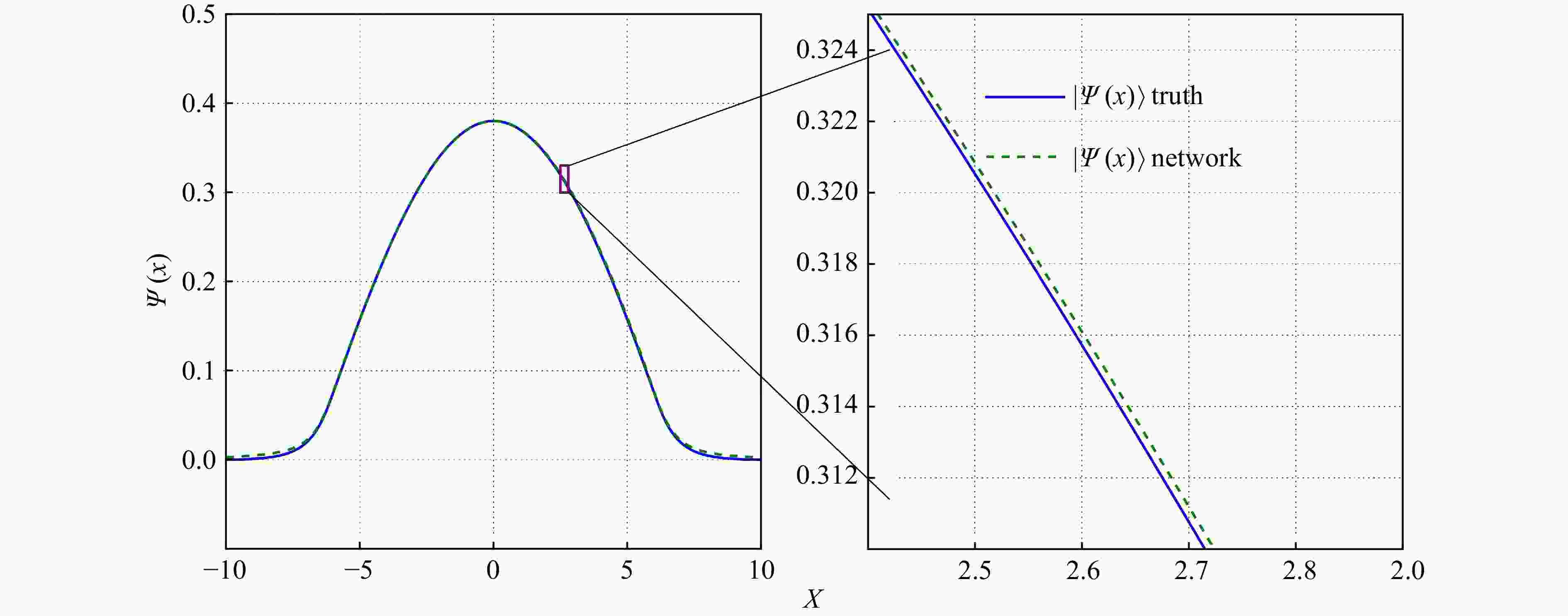
Figure 3.  The ground state wave function in the Woods-Saxon potential energy^[14].

However, compared with the results of harmonic oscillator and Woods-Saxon potential, because the ground state energy is too close to the first excitation state energy under the double-well potential, we need to appropriately increase the energy layer parameters γ so that DNN gives priority to energy optimization, in which case the ground state energy error of the double-well potential is less than 0.5% as shown in Fig. 4. In addition, we make the DNN more expressive by increasing the number of hidden layers, which brings the value of K closer to 1. The relative error of the ground state energy can be kept within 0.5% and K remains stable around 0.997 34 for the double-well potential problem. It will still maintain a high level of accuracy, although it will not be able to reach the accuracy of the first two problems.

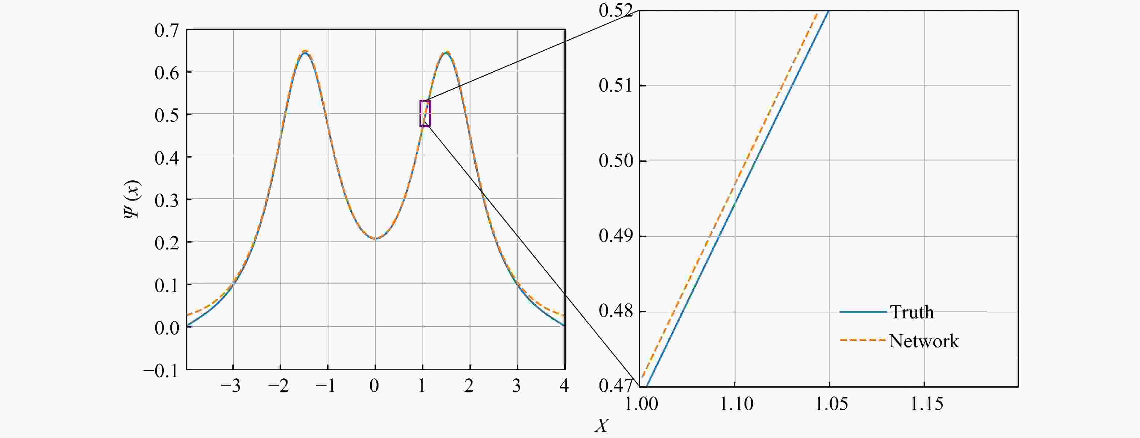
Figure 4.  The ground state wave function double-well potential.

We use DNN to fit the CDF of the ground state wave function, so that the resulting wave function automatically satisfies the normalisation and simplifies the computation. By minimising the violation of the trial wave function and the trial ground state energy $ E_0 $ to the Schrodinger equations, the variational problem is reduced to an optimization problem. This method improves the accuracy of the Schrodinger equation solution with less computation. The effectiveness of this method is confirmed by solving the harmonic oscillator, the Woods-Saxon potential and the double-well potential with small relative error.

$ E_0 = {\langle \psi | H | \psi \rangle \over \langle \psi | \psi \rangle } $ where numerical integration is required for both the numerator and the denominator in traditional variational methods for solving quantum mechanical problems. In another DNN Schrodinger solver^[9–10], the form of a trial wave function should be approximated to the exact solution for eliminating fluctuation and the initial values of the network parameters also greatly affect the optimization results. In our framework, the goal is to minimise the violation of the Schrodinger equation on the sampled spatial coordinates. The trial wave function is automatically normalized based on the constraints of the constructed neural network. The normalized ground wave function improves the efficiency of the $ E_0 $ calculation with a lower relative error. Most importantly, our algorithm is more universal and provides the possibility to solve problems that have never been solved before, because it can directly ignore the pre-training process and does not need to know any information about the exact solution before training.

There are a number of improvements that can be made to the current method. For example, active learning or coordinate sampling by the learned wave function can be used to improve training efficiency. We could improve the accuracy in solving the double-well potential problem by optimising the structure of our framework. The DNN framework will be optimized by solving the Schrodinger equation with a 3-dimensional potential. It may also open up a new way to solve many nucleon problems.

Acknowledgments This work is supported by the National Natural Science Foundation of China (Grants No. 12035006, No. 12075098), the Natural Science Foundation of Hubei Province (Grant No. 2019CFB563), Hubei Province Department of Science and Technology (Grant No. 2021BLB171).