


-
The long-term stable operation of the accelerator is an important guarantee for these studies. A very weak beam loss on the cavity will cause the failure of superconducting (SC) effect, and even irreversible damage to the accelerator system. Previous analysis shows that the failure of the SC cavity has a great contribution to the overall failure. The failure compensation of the SC cavity is crucial to ensure the stable operation of the accelerator.
Generally, the failure compensation must meet the following two conditions: (1) the output energy of beam must be stable in order to ensure the safe operation of the target and reactor; (2) Ensure beam quality and control beam loss during beam transmission. At present, the commonly compensation methods are general compensation and local compensation. The concept of the general compensation method is to use all the components downstream of the failed cavity to rematch and achieve the compensation demand[1]. As too many cavities involved in compensation, the solution space will be very complex. Especially when dealing with multi-cavity failures, the complexity of matching leads to an order of magnitude increase in compensation time. Oak Ridge National Laboratory(ORNL) tested the general compensation of the SC cavity in SNS linac[2-3]. Results show that when all the downstream components are used to compensate and rematch, the time consumed is on the order of minutes.
The local compensation method uses the elements neighboring the failure one. Four rf cavities (the two in the front and the two in the back), as well as the neighboring magnets are used to achieve the compensation. Comparing to the general compensation, this method can simplify the calculation and greatly save the time. However, fewer components used in compensation will inevitably lead to the problem that neighboring cavities must have extremely high redundancy to complete compensation. Institute of High Energy Physics(IHEP) proposed the redundancy for the
$ E_{\rm{peak}} $ (peak surface electric field) and the power should be 30% and 69% more[4]. Thus, the project cost will be dramatically increased. In addition, when the beam energy is low, considering the constraints of the longitudinal phase shift and the acceleration efficiency, the local compensation method cannot achieve the desired effect. Furthermore, local compensation can not be used for beam energy lower than 10.0 MeV. The X-ADS[5], Project-X[6] and EU RISOL[7] have considered the local compensation method. But none of them solves the high power redundancy. Therefore, Project-X and EURISOL adopt dual injector hot backup method for redundant design, which greatly increase the project cost.On the basis of previous studies, a segmented compensation method is proposed in this paper. The method of segmented compensation is to rematch the beam near the failed cavity, and compensate the energy as much as possible in consideration of economy and engineering feasibility. If the energy is not 100% compensated near the failed cavity, any downstream cavities will be used for further energy compensation. This method fully combines the advantages of local and general compensation. In this paper, the CiADS virtual accelerator, of which implemented with TraceWin software[8], are treated as an sample. And artificial intelligence algorithms[9] is applied to simulate the failure compensation of the low-energy SC cavity. Compared with other optimization algorithms, the artificial intelligence algorithm can obtain effective representations from high-dimensional sensory input and use them to promote past experience to new situations. The paper is organized as follows: Section II is a brief introduction of the physical method and numerical method used in this paper. Results and discussion are in Section III. A summary is given in Section IV.
-
The transmission process of the beam in the accelerator can be described by a matrix model, and the beam can be expressed as a
$ \sigma $ matrix:$$ \sigma = n\cdot Emi{t_{{\rm{rms}}}}\cdot \left[ {\begin{array}{*{20}{c}} {{{\tilde x}^2}}&{\overline {xx'} }&{\overline {xy} }&{\overline {xy'} }&{\overline {xz} }&{\overline {x\delta } }\\ {\overline {xx'} }&{{\tilde{x}'^{\,2}}}&{\overline {x'y} }&{\overline {x'y'} }&{\overline {x'z} }&{\overline {x'\delta } }\\ {\overline {xy} }&{\overline {x'y} }&{{{\tilde y}^2}}&{\overline {yy'} }&{\overline {yz} }&{\overline {y\delta } }\\ {\overline {xy'} }&{\overline {x'y'} }&{\overline {yy'} }&{{{\tilde {y'}}^2}}&{\overline {y'z} }&{\overline {y'\delta } }\\ {\overline {xz} }&{\overline {x'z} }&{\overline {yz} }&{\overline {y'z} }&{{{\tilde z}^2}}&{\overline {z\delta } }\\ {\overline {x\delta } }&{\overline {x'\delta } }&{\overline {y\delta } }&{\overline {y'\delta } }&{\overline {z\delta } }&{{{\tilde \delta }^2}} \end{array}} \right],$$ (1) where
$ n = 5 $ for the bunched beam,$ n = 4 $ for the continuous beam and$ Emit_{\rm{rms}} $ is the rms-emittance;$ x $ ,$ y $ ,$ z $ are beam positions in$ X,\; Y,\; Z $ directions and$ x'(p_x/p_z) $ ,$ y'(p_y/p_z) $ ,$ \delta(\varDelta p/p) $ are beam divergences in$ X,\; Y,\; Z $ directions. If we use$ \omega $ and$ \nu $ for$ x $ ,$ x' $ ,$ y $ ,$ y' $ ,$ z $ or$ \delta $ ,$ \tilde{\omega} $ is the standard deviation of$ \omega $ and$ \overline{\omega\nu} $ is the covariance of$ \omega $ and$ \nu $ . The components of the accelerator can also be represented by a transmission matrix:In this article, we choose the half wave resonance 010 type cavity (HWR010) of CiADS SC section as an example to study the compensation effect of the segmented failure compensation method in the low-energy SC section. From the matrix in Table 1, it can be seen that the cavity
$ E_{\rm{peak}} $ , phase and magnetic field strength of the solenoid affect the value of the matrix element in the corresponding transmission matrix.Table 1. The matrix of components of the accelerator.
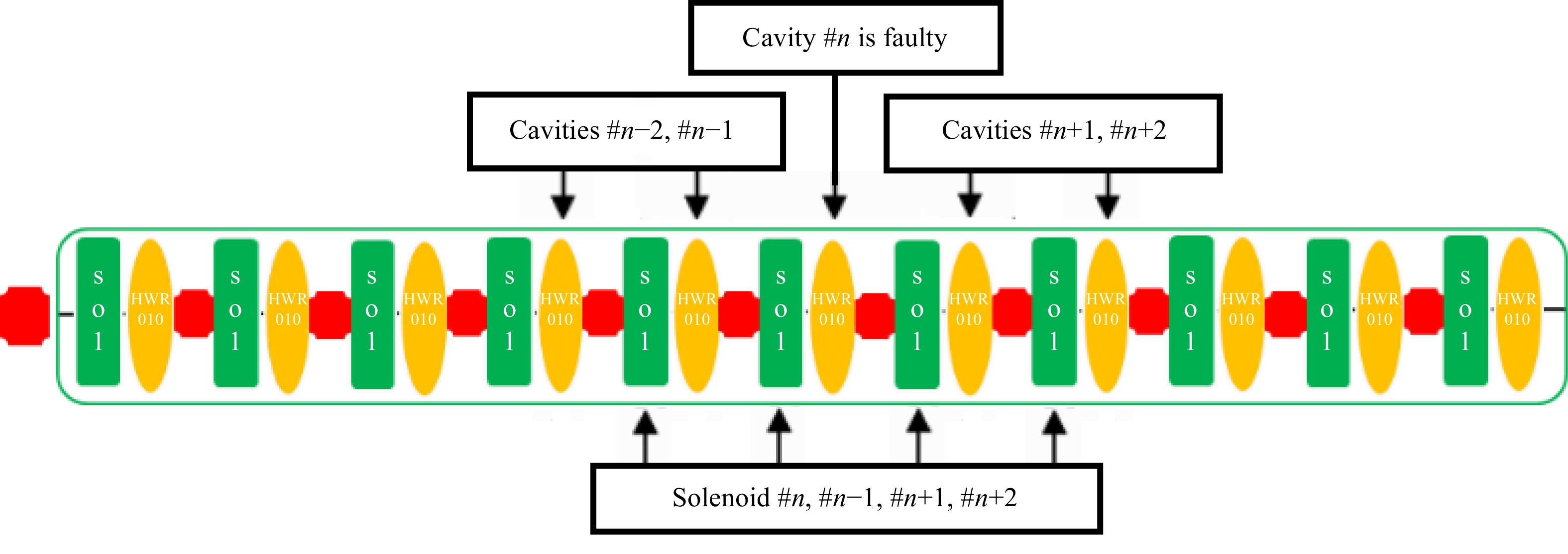
Component Matrix Drift $ \left[ {\begin{array}{*{20}{c}} 1&{\varDelta s}&0&0&0&0\\ 0&1&0&0&0&0\\ 0&0&1&{\varDelta s}&0&0\\ 0&0&0&1&0&0\\ 0&0&0&0&1&{\frac{{\varDelta s}}{{{\gamma ^2}}}}\\ 0&0&0&0&0&1 \end{array}} \right]$ Solenoid $\begin{array}{c} \left[ {\begin{array}{*{20}{c}} {{{\cos }^2}(k\varDelta s)}&{\frac{{\sin (k\varDelta s)\cos (k\varDelta s)}}{k}}&{\sin (k\varDelta s)\cos (k\varDelta s)}&{\frac{{{{\sin }^2}(k\varDelta s)}}{k}}&0&0\\ { - k\sin (k\varDelta s)\cos (k\varDelta s)}&{{{\cos }^2}(k\varDelta s)}&{ - k{{\sin }^2}(k\varDelta s)}&{\sin (k\varDelta s)\cos (k\varDelta s)}&0&0\\ { - \sin (k\varDelta s)\cos (k\varDelta s)}&{ - \frac{{{{\sin }^2}(k\varDelta s)}}{k}}&{{{\cos }^2}(k\varDelta s)}&{\frac{{\sin (k\varDelta s)\cos (k\varDelta s)}}{k}}&0&0\\ {k{{\sin }^2}(k\varDelta s)}&{ - \sin (k\varDelta s)\cos (k\varDelta s)}&{ - k\sin (k\varDelta s)\cos (k\varDelta s)}&{{{\cos }^2}(k\varDelta s)}&0&0\\ 0&0&0&0&1&{\frac{{\varDelta s}}{{{\gamma ^2}}}}\\ 0&0&0&0&0&1 \end{array}} \right]\\ {\rm{where}},k = \frac{B}{{2B\rho }},B\rho = \frac{{{m_0}c\beta \gamma }}{q} \end{array}$ Super Conducting Cavity $\begin{array}{c} \left[ {\begin{array}{*{20}{c}} {1 - {K^*}\frac{{{\varDelta _z}}}{2}}&{\frac{{{\varDelta _z}}}{2}\left( {1 - {K^*}\frac{{{\varDelta _z}}}{2} + \delta } \right)}&0&0&0&0\\ { - {K^*}\delta }&{ - {K^*}\delta \frac{{{\varDelta _z}}}{2} + {\delta ^2}}&0&0&0&0\\ 0&0&{1 - {K^*}\frac{{{\varDelta _z}}}{2}}&{\frac{{{\varDelta _z}}}{2}\left( {1 - {K^*}\frac{{{\varDelta _z}}}{2} + \delta } \right)}&0&0\\ 0&0&{ - {K^*}\delta }&{ - {K^*}\delta \frac{{{\varDelta _z}}}{2} + {\delta ^2}}&0&0\\ 0&0&0&0&1&{{\varDelta _z}}\\ 0&0&0&0&0&{{\delta ^2}} \end{array}} \right]\\ {\rm{where}},{\gamma _z} = {\gamma _\theta } + \frac{{|q|\frac{{{V_0}}}{L}{\varDelta _s}}}{{m{c^2}}},{K^*} = \frac{{qK{\varDelta _z}}}{{{m_0}{c^2}{{\bar \beta }^2}\bar \gamma }},\delta = \sqrt {\frac{{{{(\beta \gamma )}_\theta }}}{{{{(\beta \gamma )}_z}}}} ,\bar \gamma = \frac{{{\gamma _\theta } + {\gamma _z}}}{2},\bar \beta = \frac{{{\beta _\theta } + {\beta _z}}}{2} \end{array}$ As shown in Fig. 1, HWR010 is composed of 11 SC cavities, 11 solenoids and the drift tubes connected between them. The corresponding transmission matrix model is shown in Table 1. Once a SC cavity fails, taking cavity
$ \#5 $ for example, the nearby cavities (cavity$ \#3 $ , cavity$ \#4 $ , cavity$ \#6 $ , and cavity$ \#7 $ ) and solenoids (solenoid$ \#4 $ , solenoid$ \#5 $ , solenoid$ \#6 $ , and solenoid$ \#7 $ ) will participate in compensation.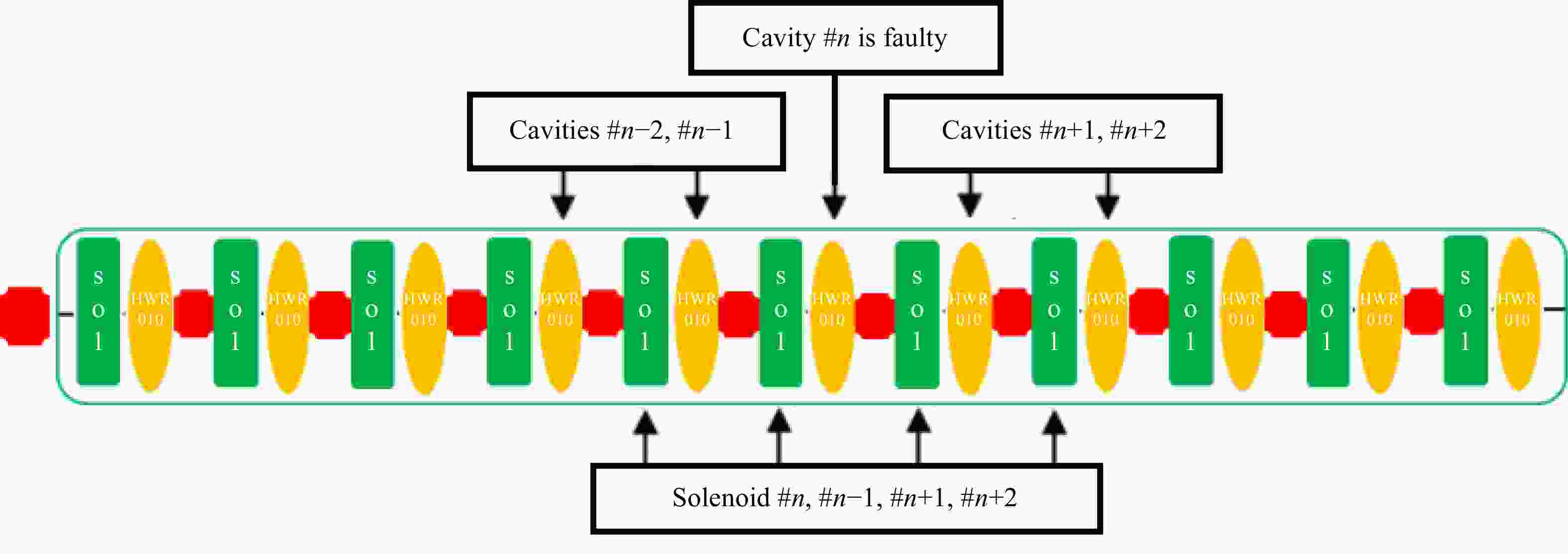
Figure 1. (color online)Layout of HWR010 segment in CiADS Linac. The red elements are the drift tubes, the green ones are SC solenoids and the yellow ones are SC cavities, respectively.
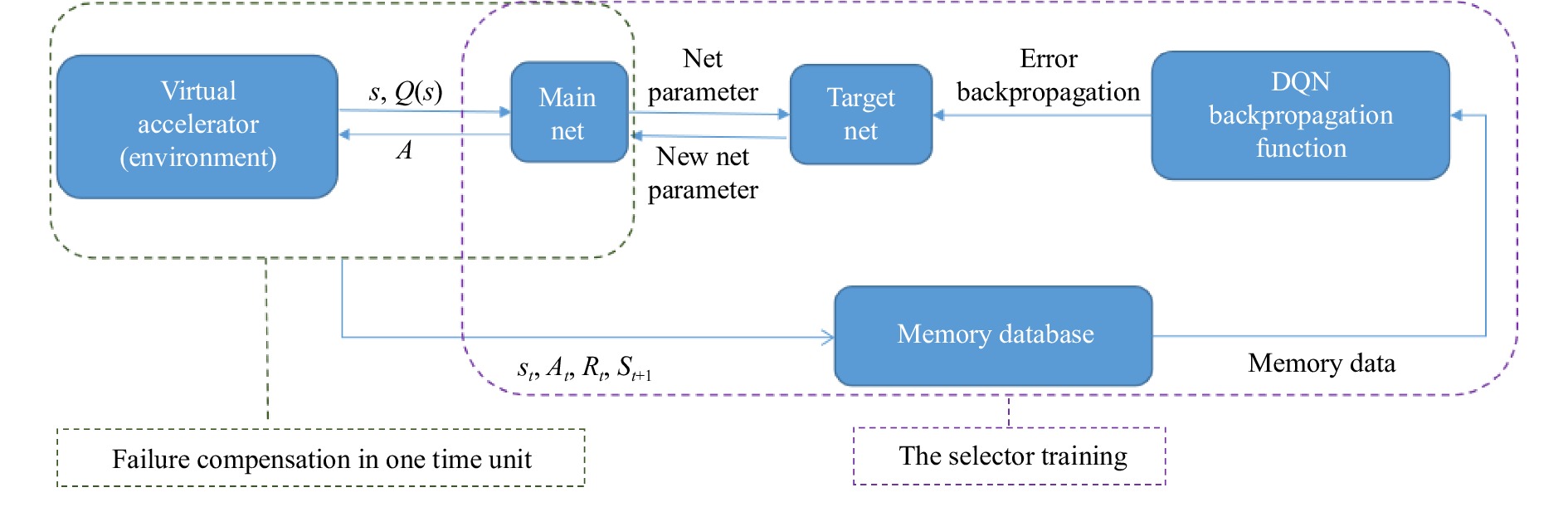
A machine learning algorithm based on reinforcement learning is used in this research and the code structure is shown in Fig. 2. In this algorithm, we first need to define the environment
$ E $ to which the algorithm is applied, and then define the environment state quantity$ s $ according to the environment$ E $ . Finally the action group$ A $ and the evaluation function$ Q(s) $ that quantitatively evaluates the state quantity$ s $ can be performed.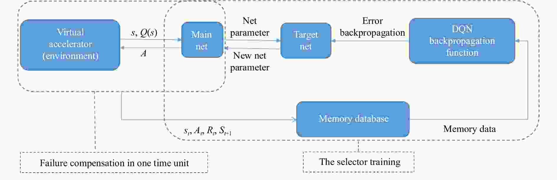
Figure 2. (color online)The code structure.
Combining this algorithm with our accelerator, the mathematical model that simulates the accelerator is actually the environment
$ E $ in which the algorithm is applied. The beam envelope is the environmental state quantity$ s $ that needs to be observed. As mentioned above, the beam envelope is a set of one-dimensional arrays corresponding to the physical location during the calculation process. If cavity$ \#n $ is faulty, the operatable elements are the solenoids$\#n-1, ~\#n, ~\#n+1,~ \#n+2$ and the SC cavities$\#n-2,~$ $ \#n-1, ~\#n+1, ~\#n+2 $ (a total of 4 SC cavities and 4 solenoids) as shown in Fig. 1. It is assumed that the increase or decrease of the magnetic filed of solenoid$ \#n-1 $ , the$ E_{\rm{peak}} $ of SC cavity$ \#n-2 $ and the phase of the SC cavity$ \#n-2 $ are defined as$a1,~ a2,~ a3, ~a4,~ a5,~ a6$ respectively; the increase or decrease of the magnetic field of solenoid$ \#n $ , the$ E_{\rm{peak}} $ of the SC cavity$ \#n-1 $ , and the phase of the SC cavity$ \#n-1 $ are respectively defined as$ a7-a12 $ . As there are 4 SC cavities and 4 solenoids, a limited action group$A\{a1,\,a2,...,a24\}$ can be constructed.During the compensation, the two sides peak envelope matching of the fault section and the smoothing of the back-end envelope (behind the fault section) of the beam are more concerned. The criteria for successful compensation are[10]: (1) The envelope near the failure cavity must satisfy the shape of "peak waist peak" (large envelope at the two sides of fault section and with a smallest envelope between them) to ensure that the envelope behind the failure cavity is smooth and convergent; (2) The outlet of each section of the cavity with different
$ \beta(v/c) $ values must meet their energy threshold. So we choose that$Q(s) =$ $ f[\varDelta x, Var(s)] $ . Where$ \varDelta x $ is the difference between the two peaks of the fault segment envelope, and$ Var(s) $ is the variance of the back-end envelope after the fault segment.When the simulated accelerator fails, the beam envelope becomes the initial fault state
$ s_0 $ . We select an action from the action group$ A $ in each time unit to act on the environment. A time unit means a iterative process that giving a new action and reading back a new state which has been indicated in Fig. 2. After$ t $ time units, the environment changes from the initial fault state$ s_0 $ to the compensated state$ s_t $ , so$s_t = f(s_0,\,A_0,...,A_t,...)$ . Where$ A_t $ is the action selected by the selector to ensure the evaluation function$ Q $ maximised. The next thing is to train the selector to ensure that the present optimal action can be chosen in different situations.The selector training process is as follows. After initializing the learning memory bank
$ D $ and the memory bank capacity$ N $ , intensive learning training is performed. At the beginning of each training, the accelerator is adjusted to the initial failure state$ s_0 $ . In each simulation compensation, the selector will select a single compensation action according to a certain probability, and then$(s_t,\, A_t,\, R_t,$ $ s_{t+1}) $ will be stored in the memory bank. Where$ s_t $ and$ s_{t+1} $ are the current state and the next state, and$ R_t $ is the real evaluation function for action$ A_t $ . Since there is a difference between the real evaluation function$ R(t) $ and prospective function$ Q(t) $ in the memory bank, the difference is back propagated for the selector training. It is expected that after several iterations, the selector can make a best selection. Physically, it can be understood as the envelope with the best evaluation will be chosen. After all these learning, when the simulated accelerator real fails, we can set up the compensation within relatively few time units which is much faster than traversing the entire solution space. -
The transverse (
$ x,\; y $ ) r.m.s. and longitudinal (phase) r.m.s. beam envelope along the longitudinal position after tracking through HWR010 section are shown in Fig. 3. Simulation is performed using multi-particle tracking code TraceWin. The beam current is 5 mA in the simulation. Without any failure of beam transport elements, the envelope is smooth: the transverse ($ x,\; y $ ) r.m.s. envelopes are less than 2 mm while the longitudinal (phase) r.m.s. envelop less than$ 5^{\circ} $ . And the normal parameters of SC cavities and solenoids changed in the simulation are provided in Table 2. Fig. 4 is the corresponding energy gain along the lattice. The beam passes through 11 drift tubes, solenoids, and SC cavities in sequence. Each time it passes through a SC cavity, the beam energy increases. The input energy is 2.0 MeV and the output energy is 8.4 MeV.
Figure 3. (color online)The beam transverse (x, y) r.m.s. and longitudinal (phase) r.m.s. envelope through HWR010 section without any failure of beam transport elements from up to down, respectively.
Table 2. The parameters of SC cavities and solenoids in the normal, single and multi-cavity failure cases.
Case Element Number Parameters #3 #4 #5 #6 #7 #8 Normal Magnetic field of Solenoid/T 3.920 8 4.161 83 4.288 39 4.172 4 4.030 8 4.125 78 Epeak of cavity/(MV/m) 19.25 23 26 26 26 27.5 Phase of cavity/$(^{\circ})$ −38 −37 −36 −35 −34 −32 #5 cavity failure Magnetic field of Solenoid/T 3.920 8 4.161 83 3.888 39 3.572 4 4.030 8 4.125 78 Epeak of cavity/(MV/m) 11.75 20 0 23.75 15 27.5 Phase of cavity/$(^{\circ})$ −36 −35 0 −34 −24 −32 #5 and #6 cavities failure Magnetic field of Solenoid/T 3.920 8 4.161 83 4.288 39 4.172 4 4.030 8 4.125 78 Epeak of cavity/(MV/m) 3 11.5 0 0 13.5 15 Phase of cavity/$(^{\circ})$ −38 −37 0 0 −34 −32 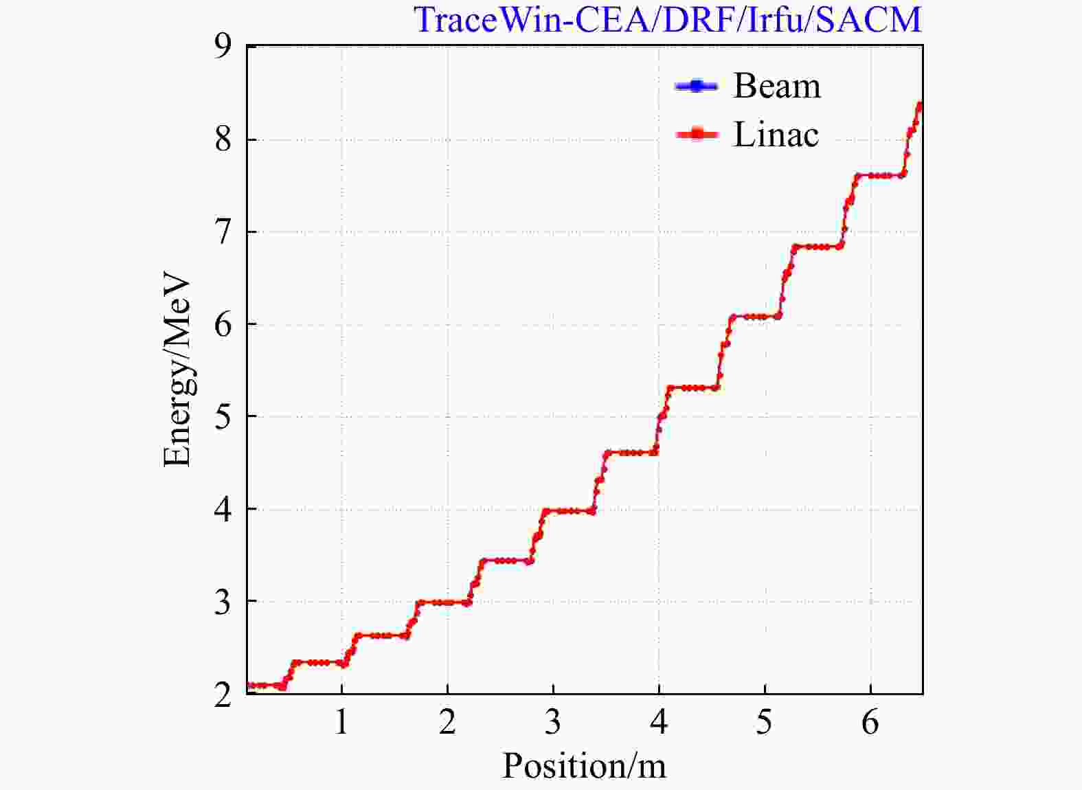
Figure 4. (color online)The beam energy along the beam position through HWR010 section without any failure of beam transport elements.
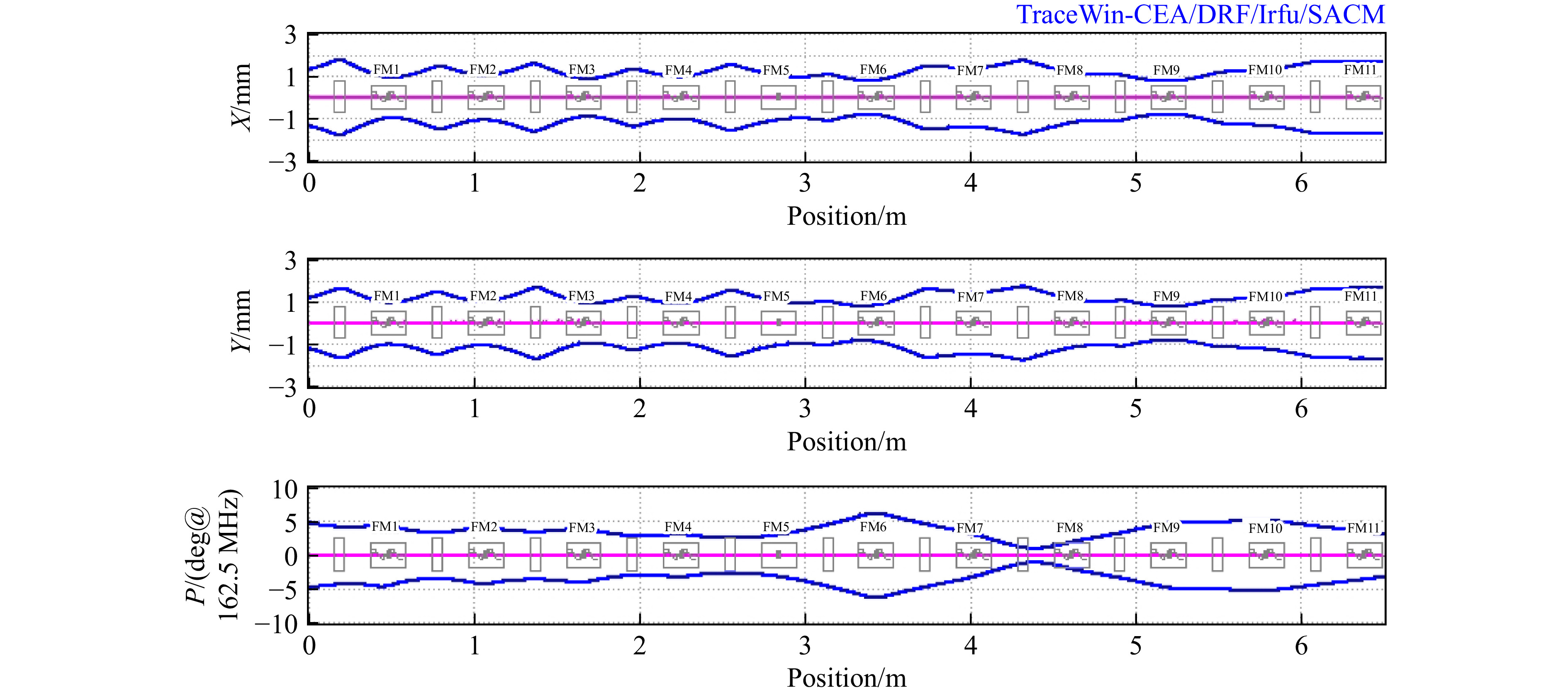
Among all kinds of failure conditions, single cavity failure is one of the most basic conditions. Fig. 5 is the beam envelopes through HWR010 in case of the failure of the fifth cavity. It can be seen that longitudinal profile of the beam blows up which results in emittance dilution and increase in beam losses, while transverse profile of the beam remains nearly unchanged. The beam envelopes after compensation of the failure cavity are shown in Fig. 6. The parameters of SC cavities and solenoids before and after compensation in the single cavity failure case are provided in Table 2. In our simulation, after modifying the super-parameters in the neural network, the program body can complete the failure compensation within 15 time units. Compared with those before failure, the end-envelope variance increment is less than 5%, while the emittance increment less than 18%. The beam can operate normally after compensation.
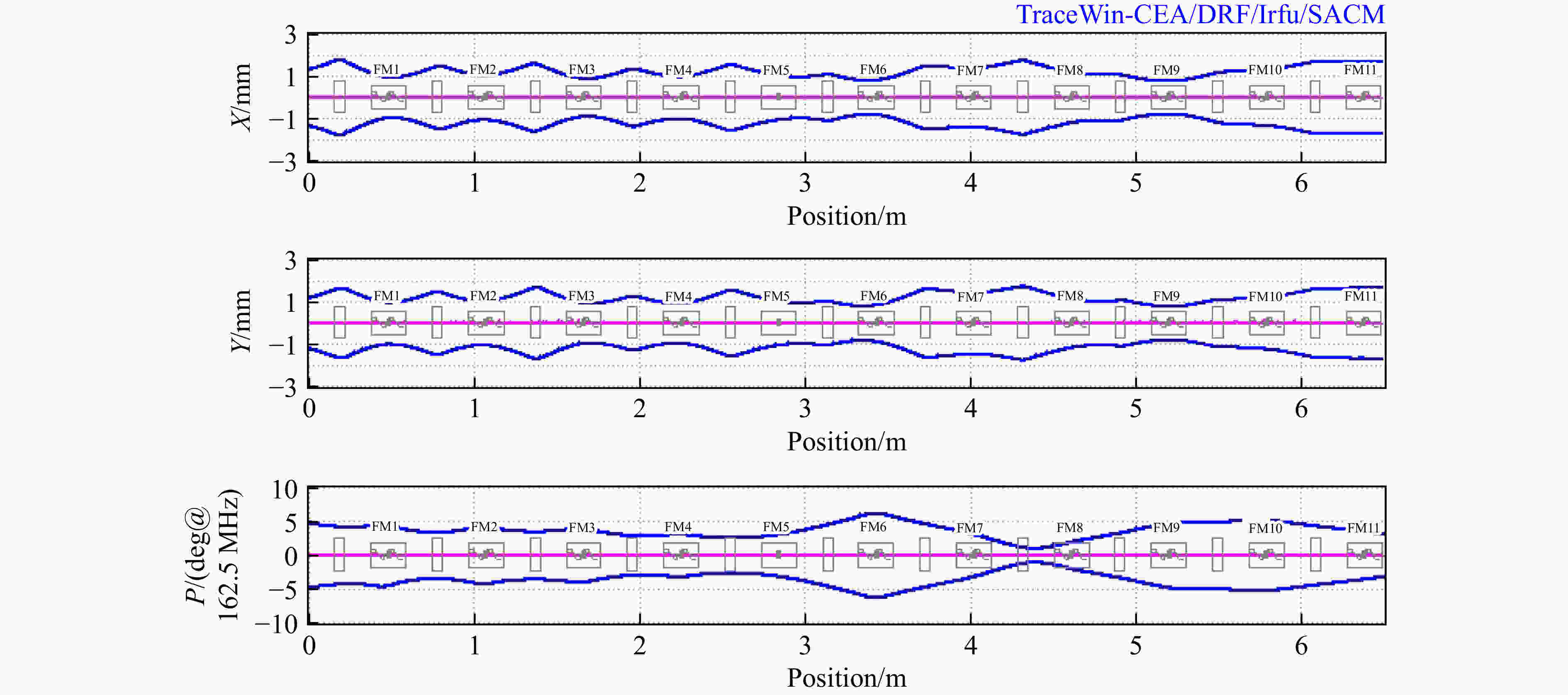
Figure 5. (color online)The beam transverse (x, y) r.m.s. and longitudinal (phase) r.m.s. envelope through HWR010 section with failure of the fifth cavity from up to down respectively.
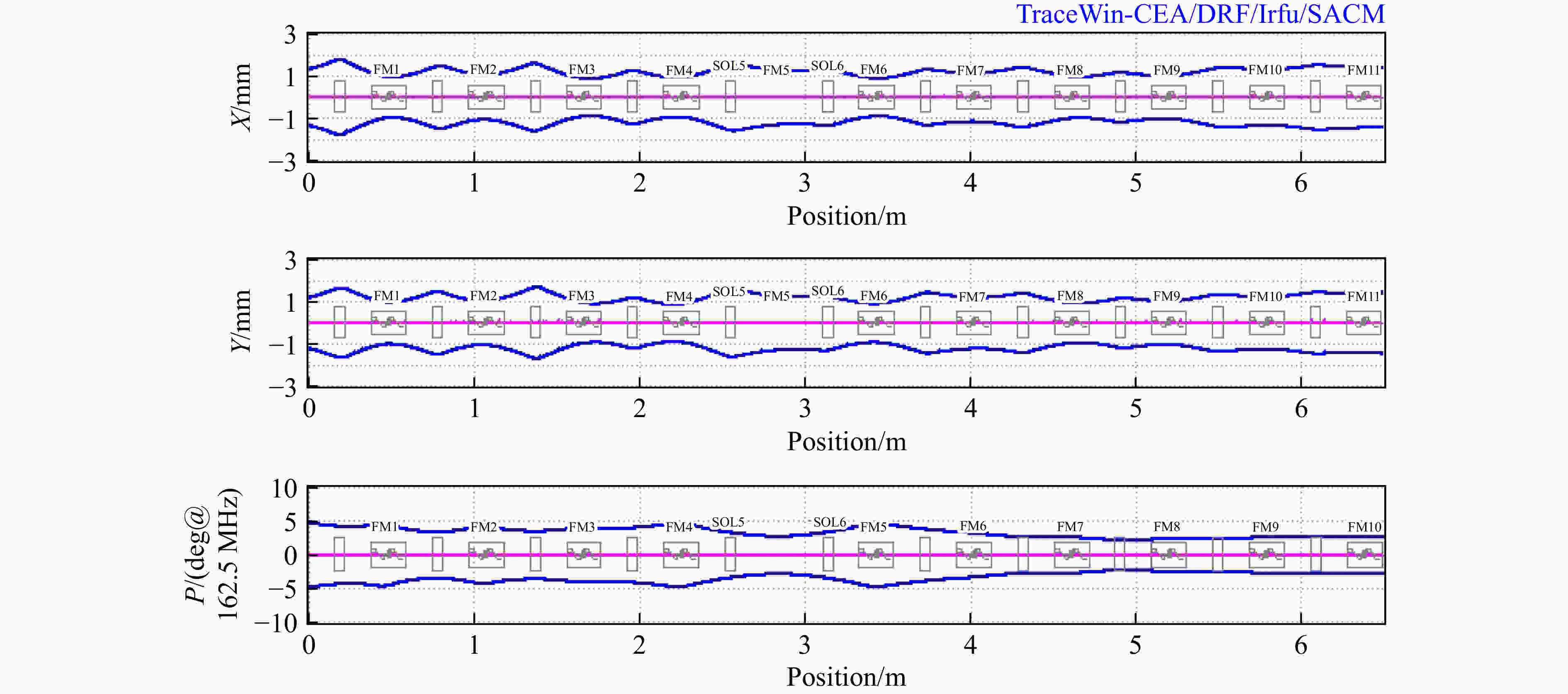
Figure 6. (color online)The beam transverse (x, y) r.m.s. and longitudinal (phase) r.m.s. envelope through HWR010 section with failure of the fifth cavity after compensation.
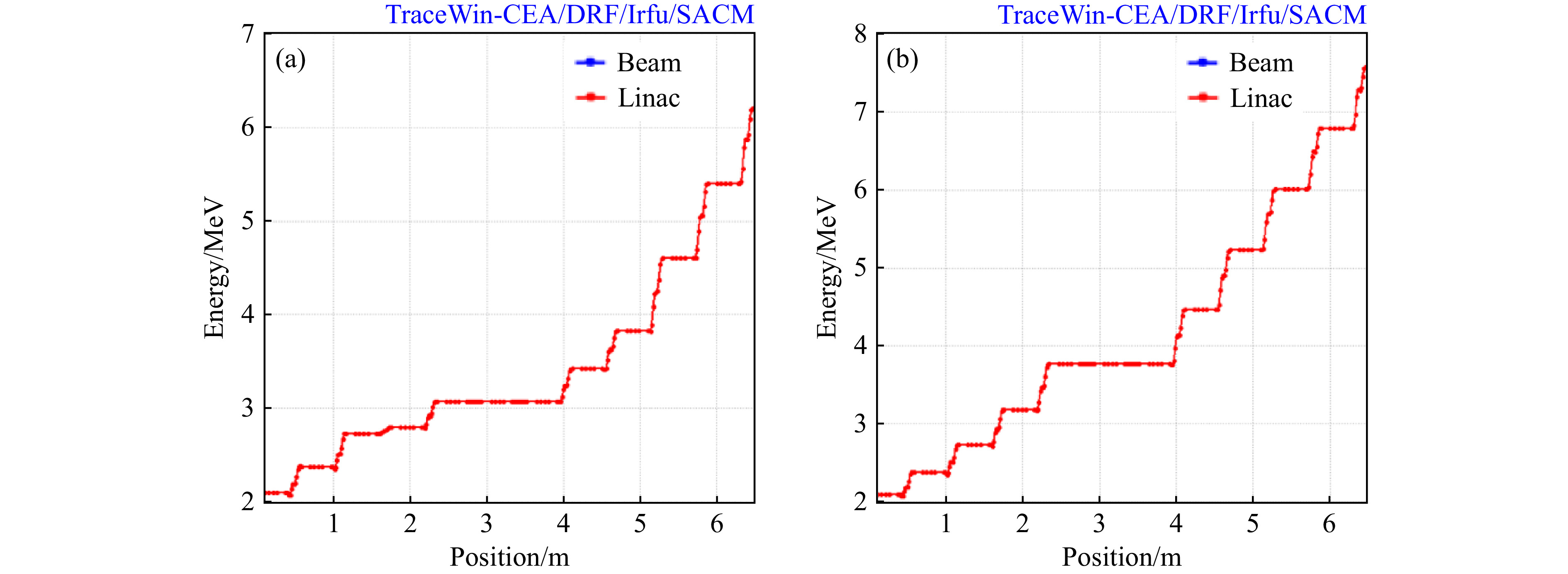
The energy gain along the lattice is shown in Fig. 7(a) and (b). Fig. 7 (a) is result before while Fig. 7(b) result after compensation. In present of the failure cavity, there are only 10 SC cavities to accelerate the beam. Before the compensation, the output energy is lower than 8.0 MeV. Then after it, the beam can achieve the designed energy and can be transported normally.
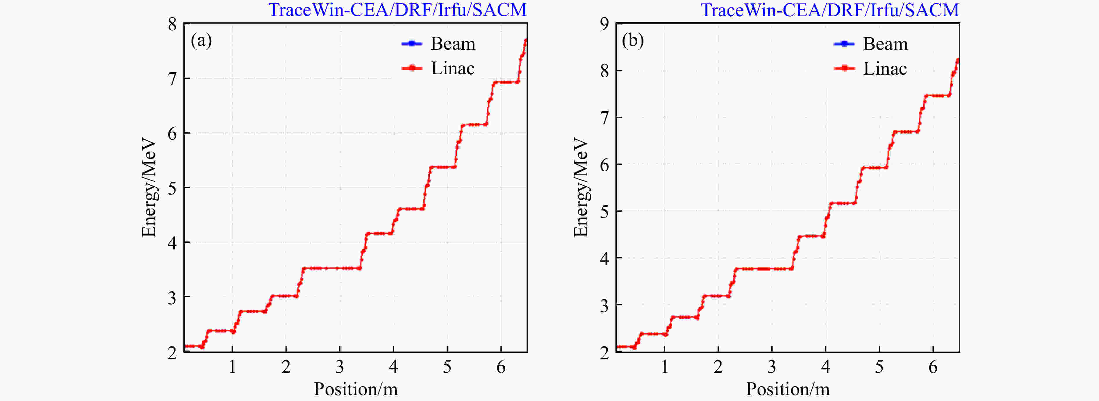
Figure 7. (color online)The beam energy along the beam position through HWR010 with failure of the fifth cavity. The cases before(a) and after(b) compensation.
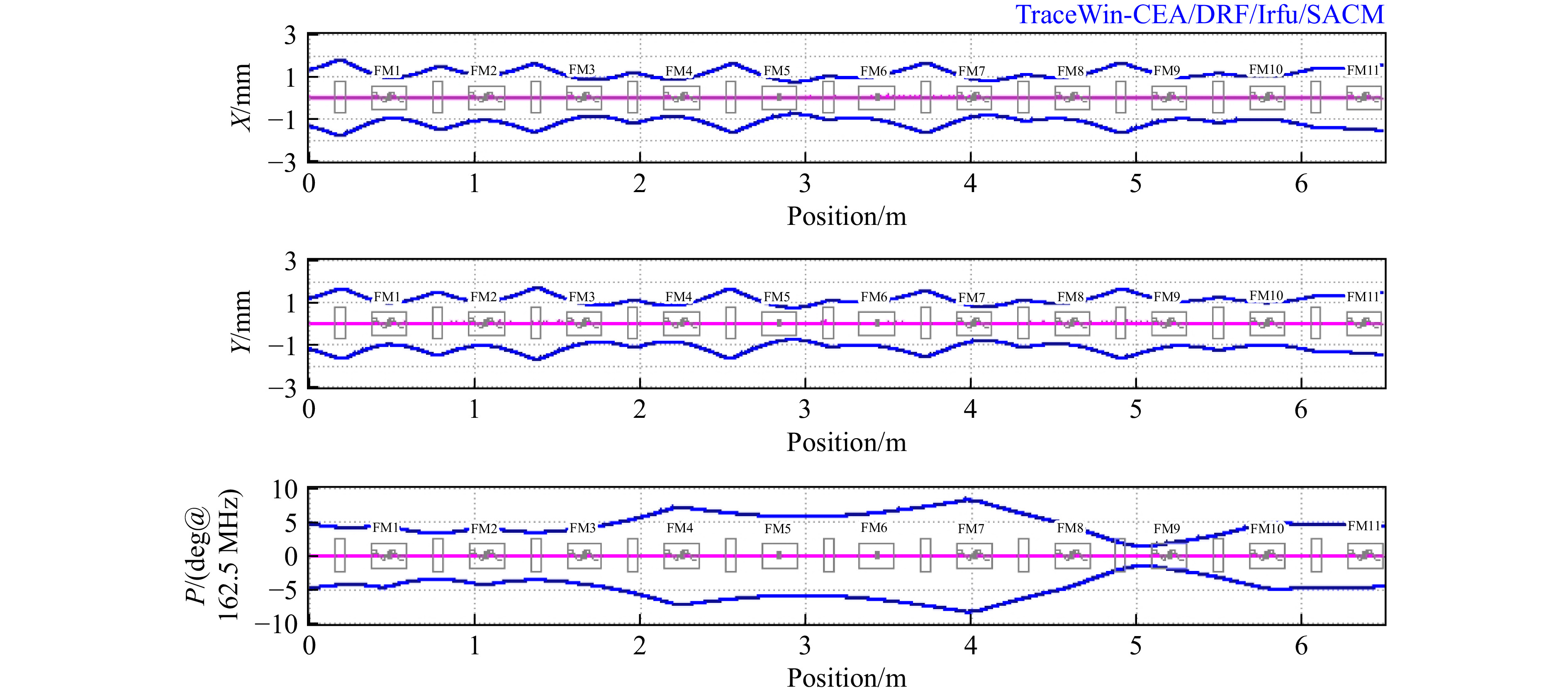
Multi-cavity compensation in the low energy section has always been a difficulty in failure compensation. Although compensation for double-cavity and single-cavity are the same in principle, the calculation of the compensation has been greatly increased due to the extended drift section. Traditional scanning methods are always limited by the step size. The method of machine learning might accomplish the dual-cavity compensation of the low energy section. We assume that the 5th and 6th SC cavities fail. The corresponding envelopes are shown in Fig. 8. Due to the serious longitudinal mismatch of the failure of two consecutive cavities, the maximum longitudinal envelope increases by more than 200%. After compensation through machine learning, the beam oscillation is reduced and the envelope is smooth as shown in Fig. 9. The parameters of SC cavities and solenoids before and after compensation in the multi-cavity failure case are provided in Table 2. Although the longitudinal envelope is still significantly increased compared with normal operation, it can already be guaranteed the beam transmitted in the HWR010 section.

Figure 8. (color online)The beam transverse (x, y) r.m.s. and longitudinal (phase) r.m.s. envelope through HWR010 section with failure of two consecutive cavities from up to down respectively.
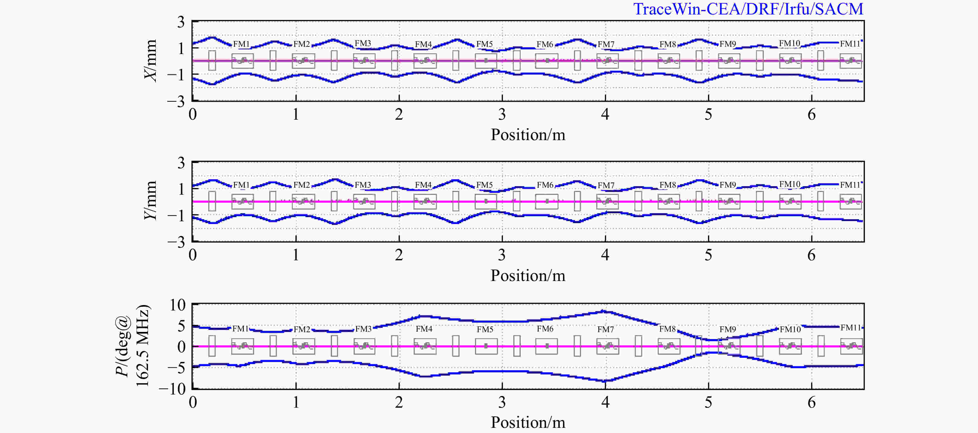
Figure 9. (color online)The beam transverse (x, y) r.m.s. and longitudinal (phase) r.m.s. envelope through HWR010 section with failure of two consecutive cavities after compensation.
The energy gain along the lattice is shown in Fig. 10(a) and (b). Fig. 10(a) is result before while Fig. 10(b) result after compensation. Due to the simultaneous failure of the two SC cavities, the energy gain is only about 6.3 MeV. After compensation, the matching energy reaches up to 7.6 MeV. Although still lower than the design energy, it reaches the SC cavity energy threshold. As mentioned above, since the simulation section is only the front 6.5m of the CiADS SC linac, further longitudinal focusing and energy compensation can be easily completed by other subsequent cavities[10].
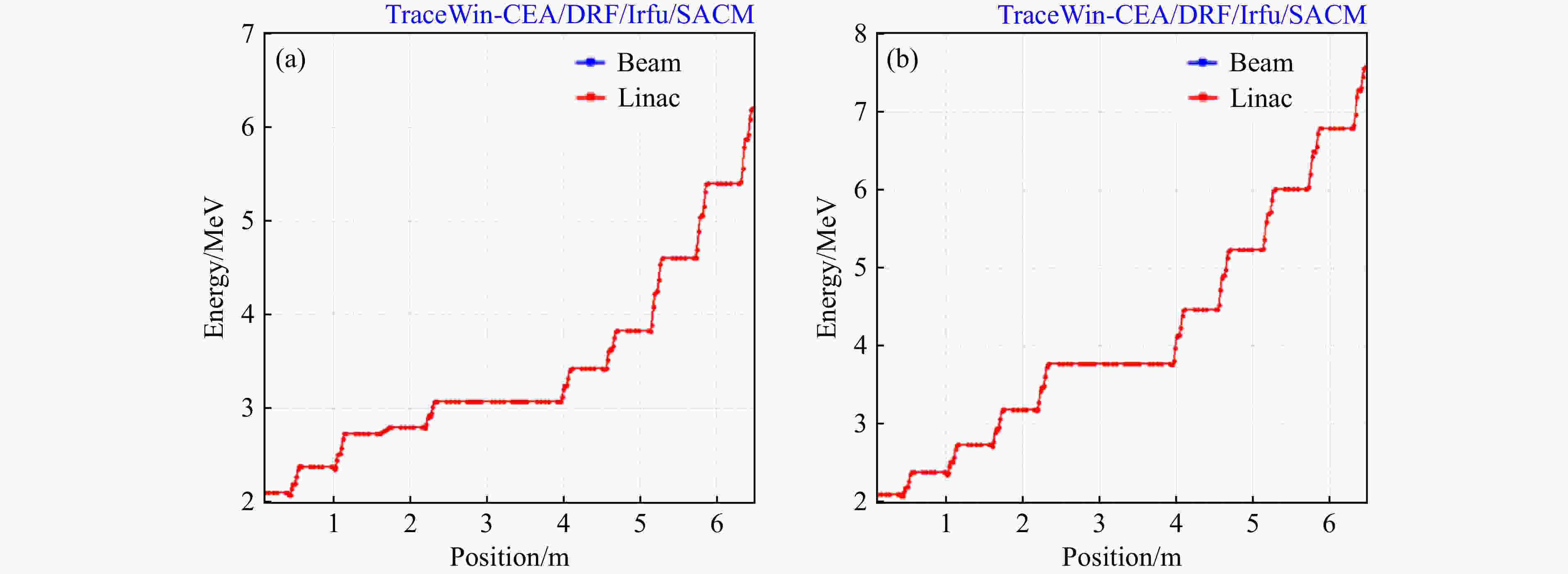
Figure 10. (color online)The beam energy along the beam position through HWR010 section with failure of two consecutive cavities. The cases before(a) and after(b) compensation.
-
In this article, the segmented failure compensation on HWR010 section of CiADS is tested by a network-based machine learning algorithm. Simulations show that for a single cavity failure, the failure can be completely compensated within 15 time units after learning. Both the envelope and energy are sufficient for effective beam transmission. For the double cavity failure case, the beam matching can still be completed in the SC section to make the envelope smooth. However, due to the simultaneous failure of the two SC cavities, the matching energy is lower than the design energy. According to the idea of segmented compensation, the energy compensation can be completed by the subsequent SC section to avoid the extremely high redundancy. Compared with the previous compensation scheme, the segmented compensation can effectively compensate the failure of the SC cavity in the low energy section, keep the output energy of beam stable, ensure beam quality, control engineering cost and reduce hardware requirements. Acknowledgments We would like to express special thanks to Dr. Qi Xin for the useful discussion. It is supported by the Youth Innovation Promotion Association, CAS(Grant No. 2018452), the National Natural Science Foundation of China(Grant No. 11775282), and Large Research Infrastructures "China initiative Accelerator Driven System"(Grant No. 2017-000052-75-01-000590).
Research on Segmented Failure Compensation of Superconducting Section in Linear Accelerator by Artificial Intelligence Algorithm
-
摘要: 强流直线加速器的长时间稳定运行是该领域的难点和前沿课题之一。以加速器驱动嬗变研究装置(CiADS)的加速器为例,利用TraceWin软件模拟的虚拟加速器数据,提出了基于人工智能算法的超导腔失效的分段故障补偿方法。当有腔体故障时,故障腔的相邻器件将用于重新匹配束流包络,而所有下游腔均可用于补偿束流能量。与传统的优化方法相比,该方法可实现低能耗的超导腔段的故障补偿,具有计算速度快、普适性强等优点,为实际应用器件故障补偿提供了新的可行性。Abstract: Long-term stable operation is one of difficult and frontier topics in the field of high-current linear accelerators. In this article, taking the China initiative Accelerator Driven System(CiADS) accelerator as an example, of whose virtual model implemented with TraceWin software by using simulation data, a segmented failure compensation method of superconducting(SC) cavity by artificial intelligence algorithm has been proposed. The neighboring elements of the failure cavities are used to rematch the beam envelope, while all the downstream cavities are used to compensate the beam energy. Compared with traditional optimization methods, this research can realize the failure compensation of low energy SC section, and has the advantages of fast calculation speed and strong versatility. It provides new feasibility for the practical application of component failure compensation.
-
Figure 1. (color online)Layout of HWR010 segment in CiADS Linac. The red elements are the drift tubes, the green ones are SC solenoids and the yellow ones are SC cavities, respectively.
Figure 3. (color online)The beam transverse (x, y) r.m.s. and longitudinal (phase) r.m.s. envelope through HWR010 section without any failure of beam transport elements from up to down, respectively.
Figure 4. (color online)The beam energy along the beam position through HWR010 section without any failure of beam transport elements.
Figure 5. (color online)The beam transverse (x, y) r.m.s. and longitudinal (phase) r.m.s. envelope through HWR010 section with failure of the fifth cavity from up to down respectively.
Figure 6. (color online)The beam transverse (x, y) r.m.s. and longitudinal (phase) r.m.s. envelope through HWR010 section with failure of the fifth cavity after compensation.
Figure 7. (color online)The beam energy along the beam position through HWR010 with failure of the fifth cavity. The cases before(a) and after(b) compensation.
Figure 8. (color online)The beam transverse (x, y) r.m.s. and longitudinal (phase) r.m.s. envelope through HWR010 section with failure of two consecutive cavities from up to down respectively.
Figure 9. (color online)The beam transverse (x, y) r.m.s. and longitudinal (phase) r.m.s. envelope through HWR010 section with failure of two consecutive cavities after compensation.
Figure 10. (color online)The beam energy along the beam position through HWR010 section with failure of two consecutive cavities. The cases before(a) and after(b) compensation.
Table 1. The matrix of components of the accelerator.
Component Matrix Drift $ \left[ {\begin{array}{*{20}{c}} 1&{\varDelta s}&0&0&0&0\\ 0&1&0&0&0&0\\ 0&0&1&{\varDelta s}&0&0\\ 0&0&0&1&0&0\\ 0&0&0&0&1&{\frac{{\varDelta s}}{{{\gamma ^2}}}}\\ 0&0&0&0&0&1 \end{array}} \right]$ Solenoid $\begin{array}{c} \left[ {\begin{array}{*{20}{c}} {{{\cos }^2}(k\varDelta s)}&{\frac{{\sin (k\varDelta s)\cos (k\varDelta s)}}{k}}&{\sin (k\varDelta s)\cos (k\varDelta s)}&{\frac{{{{\sin }^2}(k\varDelta s)}}{k}}&0&0\\ { - k\sin (k\varDelta s)\cos (k\varDelta s)}&{{{\cos }^2}(k\varDelta s)}&{ - k{{\sin }^2}(k\varDelta s)}&{\sin (k\varDelta s)\cos (k\varDelta s)}&0&0\\ { - \sin (k\varDelta s)\cos (k\varDelta s)}&{ - \frac{{{{\sin }^2}(k\varDelta s)}}{k}}&{{{\cos }^2}(k\varDelta s)}&{\frac{{\sin (k\varDelta s)\cos (k\varDelta s)}}{k}}&0&0\\ {k{{\sin }^2}(k\varDelta s)}&{ - \sin (k\varDelta s)\cos (k\varDelta s)}&{ - k\sin (k\varDelta s)\cos (k\varDelta s)}&{{{\cos }^2}(k\varDelta s)}&0&0\\ 0&0&0&0&1&{\frac{{\varDelta s}}{{{\gamma ^2}}}}\\ 0&0&0&0&0&1 \end{array}} \right]\\ {\rm{where}},k = \frac{B}{{2B\rho }},B\rho = \frac{{{m_0}c\beta \gamma }}{q} \end{array}$ Super Conducting Cavity $\begin{array}{c} \left[ {\begin{array}{*{20}{c}} {1 - {K^*}\frac{{{\varDelta _z}}}{2}}&{\frac{{{\varDelta _z}}}{2}\left( {1 - {K^*}\frac{{{\varDelta _z}}}{2} + \delta } \right)}&0&0&0&0\\ { - {K^*}\delta }&{ - {K^*}\delta \frac{{{\varDelta _z}}}{2} + {\delta ^2}}&0&0&0&0\\ 0&0&{1 - {K^*}\frac{{{\varDelta _z}}}{2}}&{\frac{{{\varDelta _z}}}{2}\left( {1 - {K^*}\frac{{{\varDelta _z}}}{2} + \delta } \right)}&0&0\\ 0&0&{ - {K^*}\delta }&{ - {K^*}\delta \frac{{{\varDelta _z}}}{2} + {\delta ^2}}&0&0\\ 0&0&0&0&1&{{\varDelta _z}}\\ 0&0&0&0&0&{{\delta ^2}} \end{array}} \right]\\ {\rm{where}},{\gamma _z} = {\gamma _\theta } + \frac{{|q|\frac{{{V_0}}}{L}{\varDelta _s}}}{{m{c^2}}},{K^*} = \frac{{qK{\varDelta _z}}}{{{m_0}{c^2}{{\bar \beta }^2}\bar \gamma }},\delta = \sqrt {\frac{{{{(\beta \gamma )}_\theta }}}{{{{(\beta \gamma )}_z}}}} ,\bar \gamma = \frac{{{\gamma _\theta } + {\gamma _z}}}{2},\bar \beta = \frac{{{\beta _\theta } + {\beta _z}}}{2} \end{array}$  下载: 导出CSV
Table 2. The parameters of SC cavities and solenoids in the normal, single and multi-cavity failure cases.
Case Element Number Parameters #3 #4 #5 #6 #7 #8 Normal Magnetic field of Solenoid/T 3.920 8 4.161 83 4.288 39 4.172 4 4.030 8 4.125 78 Epeak of cavity/(MV/m) 19.25 23 26 26 26 27.5 Phase of cavity/$(^{\circ})$ −38 −37 −36 −35 −34 −32 #5 cavity failure Magnetic field of Solenoid/T 3.920 8 4.161 83 3.888 39 3.572 4 4.030 8 4.125 78 Epeak of cavity/(MV/m) 11.75 20 0 23.75 15 27.5 Phase of cavity/$(^{\circ})$ −36 −35 0 −34 −24 −32 #5 and #6 cavities failure Magnetic field of Solenoid/T 3.920 8 4.161 83 4.288 39 4.172 4 4.030 8 4.125 78 Epeak of cavity/(MV/m) 3 11.5 0 0 13.5 15 Phase of cavity/$(^{\circ})$ −38 −37 0 0 −34 −32
下载: 导出CSV
-
[1] BIARROTTE J L, URIOT D. Physical Review Special Topics - Accelerators and Beams, 2008, 11: 072803. [2] GALAMBOS J, HENDERSON S, ZHANG Y. 2006: MOP057 [EB/OL]. [2021-05-15]. https://accelconf.web.cern.ch/l06/PAPERS/MOP057.PDF. [3] KIM S, RIDGE O. 2008: MO103[EB/OL]. [2021-05-15]. https://epaper.kek.jp/LINAC08/papers/mo103.pdf. [4] SUN B, YAN F, PEI S L, et al. Chinese Physics C, 2015, 39: 117003. [5] BIARROTTE J, NOVATI M, PIERINI P, et al. AIP Conference Proceedings, 2005, 773: 99. [6] A.SAINI, K.RANJAN. 2011: WEP006[EB/OL]. [2021-05-15].https://accelconf.web.cern.ch/PAC2011/papers/wep006.pdf. [7] BIARROTTE J L. High Power CW Superconducting Linacs for Eurisol and XADS[EB/OL]. [2021-05-15]. https://accelconf.web.cern.ch/l04/papers/tu301.pdf. [8] URIOT D. DACM Software for Accelerator Design and Simulation[EB/OL]. [2021-05-15]. http://irfu.cea.fr/Sacm/logiciels/index3.php. [9] VAN HASSELT H, GUEZ A, SILVER D. Deep Reinforcement Learning with Double Q-learning[EB/OL]. [2021-05-15]. https://dl.acm.org/doi/10.5555/3016100.3016191. [10] JIA Yongzhi, HE Yuan, WANG Zhijun, et al. Nuclear Physics Review, 2019, 36(1): 62. (in Chinese) -

 点击查看大图
计量
- 文章访问数: 466
- HTML全文浏览量: 132
- PDF下载量: 40
- 被引次数: 0


 甘公网安备 62010202000723号