


-
Heavy-ion cancer therapy (HICT) is an emerging technology with rapid development and an advanced form for cancer treatment. It is based on the Bragg's effect of the heavy-ion beams in a finite depth of the body tumour i.e., the dose deposition profile exhibits a maximum close to the ion range and then falls steeply. This suggests that the dose could be focused on the tumour and, the dose on the healthy tissue can be minimized by matching the ion energy with the tumour depth. Therefore, the precise surveillance of the Bragg peak location is a critical issue. A mismatch could lead to an under-dosage in the tumour and an over-dosage in healthy tissues.
A demonstration HICT with the complete intellectual property rights has been built by Institute of Modern Physics, Chinese Academy of Sciences in Gansu Province, China. In order to achieve the condition of medicine security, different methods for monitoring the ion range have been developed. The most common methods among them is the particle range measurements employing the positron emission tomography (PET), which detects the annihilating
$ \gamma $ -rays of positrons produced in nuclear reactions[1-3]. Another method called single-photon emission computed tomography (SPECT) has been investigated in past years to obtain the online imaging of the therapy region[4-7].In recent years, a piece of alternative equipment called Compton camera is being studied and constructed for online imaging of the
$ \gamma $ -rays in HICT. The Compton camera seems as a promising setup for prompt$ \gamma $ -ray imaging because it has a wide energy-detection range from a few hundred keV up to a few MeV[8-14]. Generally, the Compton camera comprises of multiple position-sensitive detectors, arranged in a scattering plane and an absorbing plane. It records the energies being deposited by the$ \gamma $ -rays in each plane as well as the interaction positions. Then based on the Compton kinematics, the density map for the$ \gamma $ -ray source could be constructed by imaging algorithms[15].The Compton camera uses a scattering detector to localize the track of the
$ \gamma $ -rays. This will introduce some errors while determining the actual positions and energies of interactions, and further effects the image resolution of the Compton camera. Doppler broadening also adds to the inherent limitations for the Compton camera to high resolution. This effect comes from the Compton scattering of$ \gamma $ -rays on the moving electron bound to an atom rather than on a stationary electron as the Compton equation assumed.This work aims to study the effects of the Doppler broadening on the resolution ability of the Compton camera. Hirasawa and Tomitani[16] proposed for the first time an analytical study on Doppler broadening contribution to the angular uncertain, and further demonstrate the Doppler broadening effects affecting the resolution of the imaging. Uche
$ et\; al $ .[17] also simulated the Doppler energy broadening using the Geant4 toolkit. They found an imaging resolution of 2.4 and 4.2 mm, respectively for Silicon and Germanium scatterer, for a 511-keV point-like gamma source. This value is far beyond the actual use of Compton camera in HICT. Our simulation shows that less than 1.0 mm resolution can be achieved when the voxel in the imaging space is set to 0.1 mm, considering the Doppler broadening effects only. Section 2 is the simulation method and results describing the simulation details and algorithm. Section 3 is the imaging reconstruction, and, Section 4 is the conclusion of the work. -
The simulation was performed by using the Geant4 toolkit employing the G4EMPenelopePhysics physical package, directly incorporating the atomic shell cross-section data for low energy processes. Many external reference libraries[18] have validated the low-energy Penelope package. The Compton camera geometry in this work consists of two layers of pixel array detectors. The layer close to the gamma source is called the scattering detector, and the other is an absorb detector. Each layer has an effective area of 60 mm
$ \times $ 60 mm being divided into 12$ \times $ 12 pixels, resulting the position resolution in$ XY $ plane equal to 5 mm. The distance between the two layers is 50 mm. The thickness of scattering detector and absorb detector is 10 and 20 mm, respectively. For decreasing the backward scattering effect (the Compton scattering occurred at the absorb detector)[19], the material of the scattering detector is selected as a low-$ Z $ Silicon, and the absorb detector is a high-$ Z $ Germanium. The isotropic point-like gamma source was positioned at the centre of the Compton camera field of view at a distance of 30 mm from the scattering detector.When a
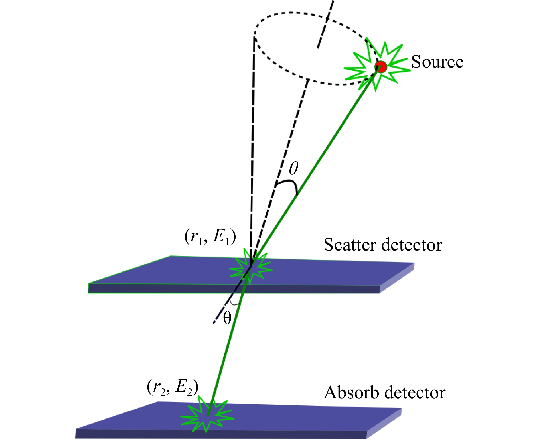
$ \gamma $ -ray with energy$ E_{0} $ emitted from the source located at${ r}_0$ is Compton scattered at point${ r}_{1}$ in the scattering detector then absorbed at point${ r}_{2}$ in the absorb detector, as shown in Fig. 1. The scattering angle$ \theta_{\rm G} $ is given directly by the geometric triangle relation,$$ \begin{array}{l} \cos\theta_{\rm G} = \dfrac{{{r}}_0{{r}}_1\cdot{{r}}_1{{r}}_2}{\mid{{r}}_0{{r}}_1\mid\cdot\mid{{r}}_1{{r}}_2\mid}. \end{array} $$ (1) Assuming the orbital electron in the scattering detector is free and at rest, the Compton formula estimates this scatter angle as
$$ \begin{array}{l} \cos\theta_{\rm C} = 1-m_{0}c^{2}\Big(\dfrac{1}{E_{2}}-\dfrac{1}{E_{0}}\Big), \end{array} $$ (2) where,
$ m_{0}c^{2} $ is the electron rest energy;$ E_{2} $ is the deposited energy in the absorb detector;$ E_{1} $ is the deposited energy in the scatter detector and$ E_0 = $ $ E_1+E_2 $ .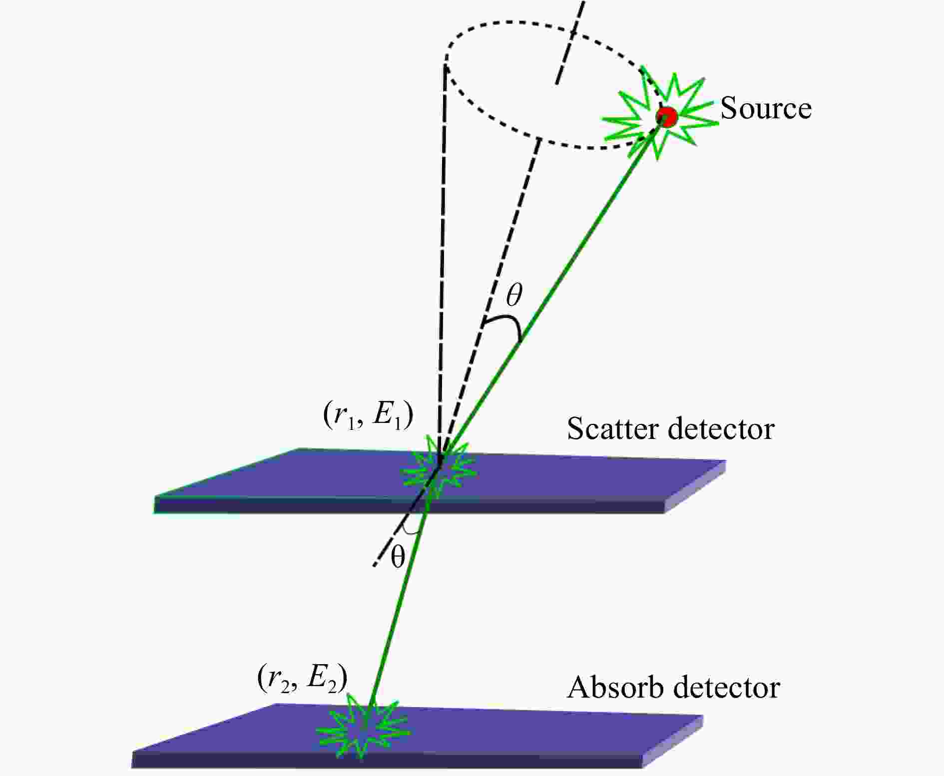
Figure 1. (color online) Schematic of a Compton camera consisting of a scattering detector and an absorb detector. The scattering angle
$ \theta $ can be constructed by the interaction positions and deposited energies according to the Compton scattering formula.Because an actual Compton scattering occurs on a moving electron bound to an atom rather than a stationary electron, both the deposited energies
$ E_{1} $ and$ E_{2} $ have physical uncertainties then the scattering angle$ \theta_{\rm C} $ is also uncertain. This effect is the so-called Doppler broadening effect. If one assumes the measuring of$ E_{1} $ ,$ E_{2} $ ,${ r}_{1}$ and${ r}_{2}$ accurately, then the$ \theta_{\rm C} $ will show a distribution centered approximately at$ \theta_{\rm G} $ . Since the G4EMPenelopPhysics package used in present work includes the atomic data for low energy process, thus the Doppler broadening effect could be studied based on the obtained deposited energies and the scattering positions.For investigating the image precision of the Compton camera, it is convenient to define the angular resolution measure (ARM) as
$$ \begin{array}{l} \theta_{\rm ARM} = \theta_{\rm C}-\theta_{\rm G}. \end{array} $$ (3) In the simulation, the values of (
${ r}_1$ ,$ E_1 $ ) and (${ r}_2$ ,$ E_2 $ ) could be tracked exactly. Then the ARM's standard deviation$ \sigma_{\rm ARM} $ will be same as that of Compton scatter angle. For re-constructing the imaging of the gamma source, it must have many true events in which each$ \gamma $ -ray is scattered once in the scattering detector and then absorbed completely in the absorb detector. The ARM distribution formed by such multiple true events represents the overall effects of the Doppler broadening on the Compton scatter angle. Therefore, the$ \sigma_{\rm ARM} $ or the full width at half maximum (FWHM) is related to the image's precision, which can be expressed based on the geometric relation,$$ \begin{array}{l} \varGamma_{{\rm image}} = \varGamma_{{\rm ARM}}\cdot\overline{\mid{{{r}}_0{{r}}_1}\mid}, \end{array} $$ (4) where
$ \overline{\mid{{{r}}_0{{r}}_1}\mid} $ represents the mean value of$ \mid{{{r}}_0{{r}}_1}\mid $ (In this work it is 30 mm).For reducing the statistical errors,
$10 ^{9} $ isotropic$ \gamma $ -rays with homology energies were simulated. Only the event that the original gamma scattered once in the scattering detector and then absorbed in the absorb detector was selected. Figure 2(a) shows the simulated Doppler broadening effects for 150-keV gamma scattered in the Silicon crystal. Here is a 2D histogram, where the y-axis represents the Compton scattering angle$ \theta_{\rm C} $ and the x-axis is the geometry angle$ \theta_{\rm G} $ . As shown, both the$ \theta_{\rm C} $ and$ \theta_{\rm G} $ are from 0° to 100°, and the$ \theta_{\rm C} $ is centred at approximately$ \theta_{\rm G} $ . Figure 2(b) shows the corresponding ARM distribution. As a comparison, the ARM simulated using the G4EMStandardPhysics model is also shown (the solid line). It can be seen from Fig. 2(b), the ARM is centered at 0° and has an obvious broadening as compared with that by using the G4EMStandardPhysics model.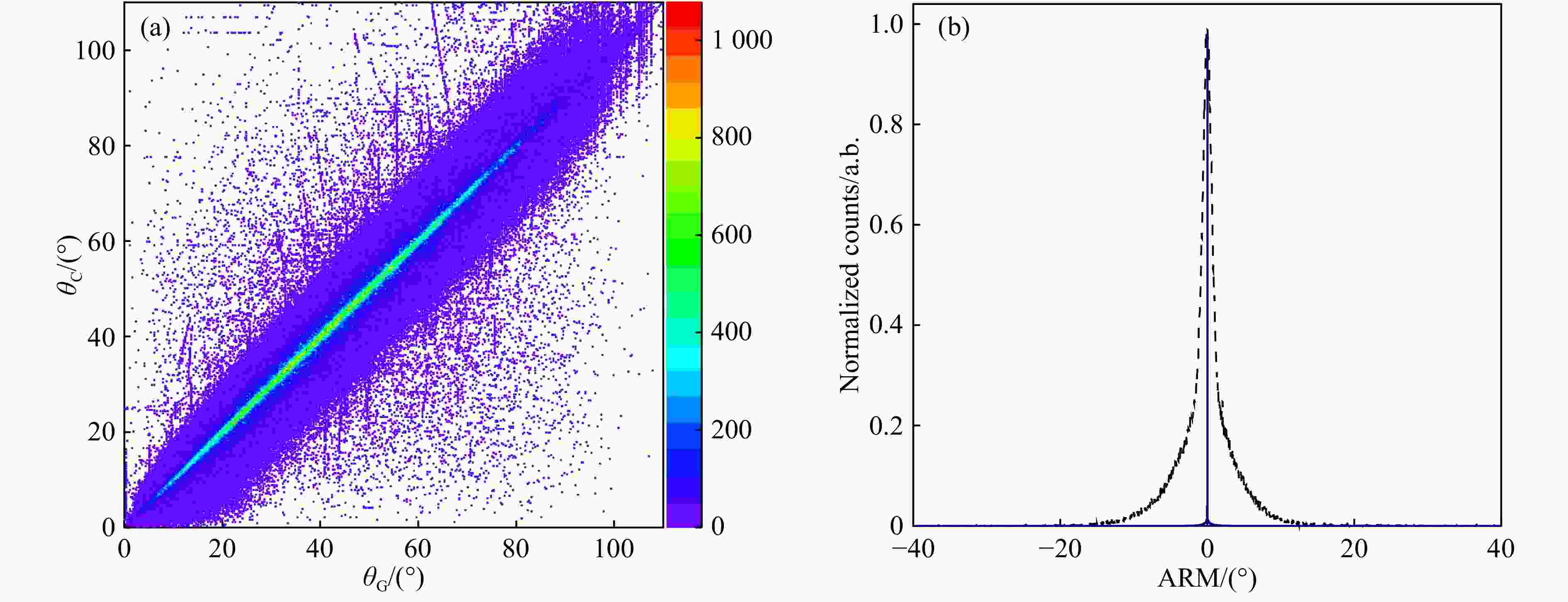
Figure 2. (color online) Statistical distribution of (a) Doppler broadening, and (b) corresponding ARM.
The FWHM of the ARM for several scattering mediums and two incident photon energies (150 and 511 keV) is summarized in Table 1. As shown, the FWHM increases with increasing the atomic number of the scattering medium and decreasing the incident energies.
Table 1. Estimation of FWHM of ARM for different scattering medium (Si, Ge, LSO and BGO) at two incident photon energies (150 and 511 keV).
Energy/keV FWHM of ARM/(°) Si Ge BGO LSO 150 1.7 2.3 – – 511 0.55 0.85 0.95 1.3 For investigating the Doppler broadening of different gamma energies in different materials, we have shown some 2D histograms for the energies transferred to the recoiled electrons by the incident gamma versus the scattering angle. Figure 3(a) and 3(b) represent 150-keV gamma scattering in Silicon and Germanium crystal, respectively. From the figure, it can be observed that there is more broadening in Ge (Germanium) than Si (Silicon). Figure 3(c) shows the 2D histogram for 511-keV
$ \gamma $ -ray in Si, which on comparison with 3(a) shows less broadening. These results illustrate that better imaging resolution is more probable at high incident energies than at low energies, and low-$ Z $ materials may be the more suitable material for making the scattering detector of the Compton camera.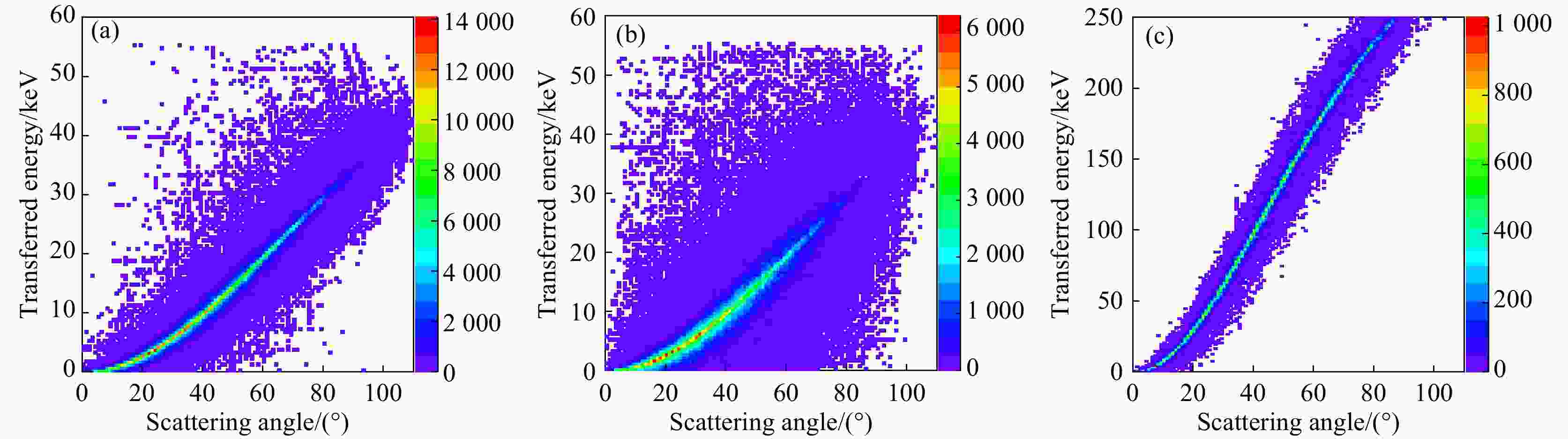
Figure 3. (color online) 2D histogram of energy-angle distribution for 150-keV gamma in (a) silicon detector and (b) germanium detector, (c) 511-keV gamma in Silicon.
-
Ideally, for any effective event, j, the gamma source must be located on a cone surface with
$ R_1 $ as the vertex,$ {{r}}_1{{r}}_2 $ as the axis, and the scattering angle$ \theta_j $ as the half-angle. In polar coordinates, it can be expressed by probability density function (Delta function) as$ F_j(\theta) = \delta(\theta-\theta_j) $ .However, the real Compton camera is an array of crystal detectors and contains a complex electronic data-acquisition system. Thus, it will bring some errors while measuring the position and energy of the
$ \gamma $ -rays. Another source of error is the Doppler effect. Therefore, the errors for the (${ r}_1$ ,$ E_1 $ ) and (${ r}_2$ ,$ E_2 $ ) from the measurements and the Doppler effects will introduce an error$ \Delta $ $ \theta_j $ for the scattering angle$ \theta_j $ . The gamma source should be located on a "hollow" cone with$ \Delta $ $ \theta_j $ as the thickness of the conical wall. In polar coordinates, the probability of the gamma source on the hollow cone can be described by a distribution function, for example, the Lorentz function,$$ \begin{array}{l} F_j(\theta, \Delta\theta_j) = \dfrac{1}{\pi}\dfrac{\Delta\theta_j}{(\theta-\theta_j)^2+(\Delta\theta_j)^2}. \end{array} $$ (5) In the imaging reconstruction, the location space of the gamma source is called the imaging space. We divide the imaging space into several small cubes with equal spacing, and each cube is called a voxel. For example, suppose that the size of the imaging space is 50 mm
$ \times $ 50 mm$ \times $ 50 mm, and the size of a voxel is 0.5 mm$ \times $ 0.5 mm$ \times $ 0.5 mm, thus dividing the imaging space into$ 10^6 $ voxels.The "hollow" cone intersects with some voxels, and the weight for any intersecting voxel, i, can be obtained by integrating the Eq. (5) over this voxel,
$ i.e $ .,$$ \begin{array}{l} W_{ij} = \int\nolimits_VF_j(\theta, \Delta\theta_j){\rm d}V_i, \end{array} $$ (6) where
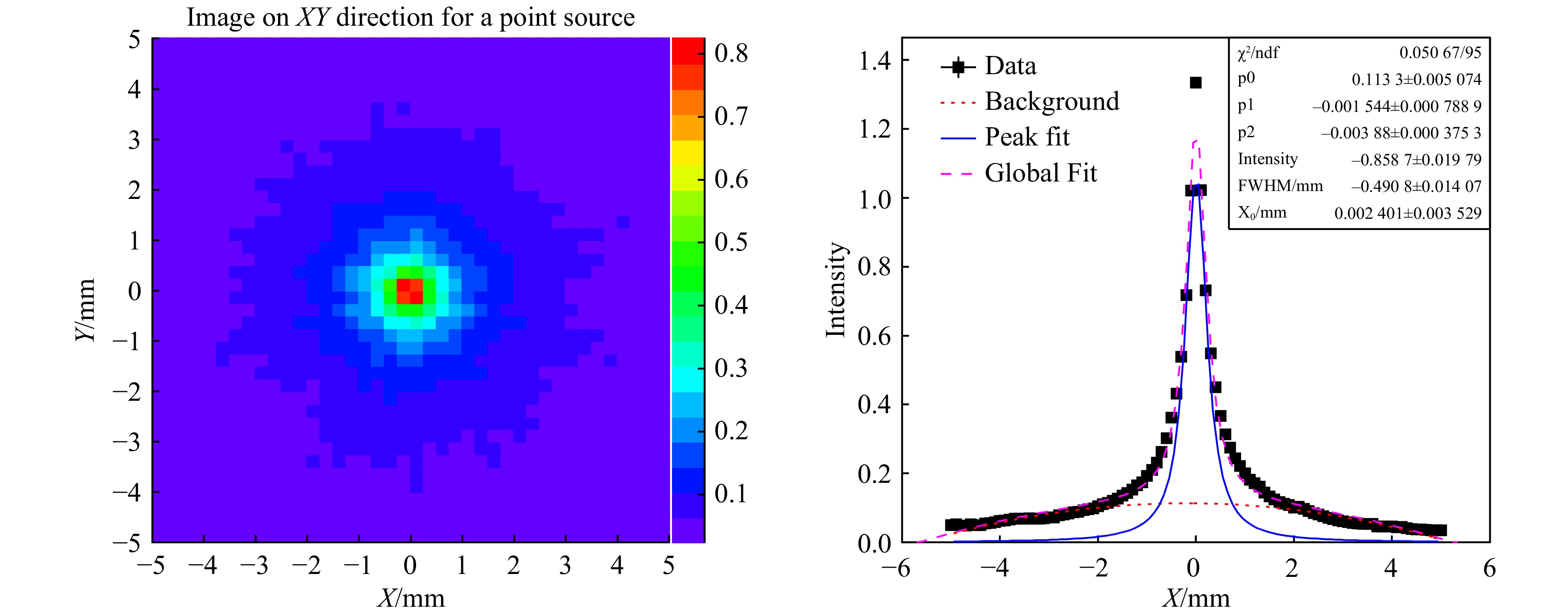
$ {\rm d}V_i $ is the volume element in the intersections between the "hollow" cone with the i-th voxel, and to obtain the total weight of each voxel, all the effective events$ \sum_j $ $ W_{ij} $ are being summed up. Thus suggesting the probability of the gamma source in each voxel to be proportional to the total weight.Figure 4 shows the imaging of a point-like source for 150-keV
$ \gamma $ -ray in Silicon material by using the algorithm discussed above. It should be noted that only the error from Doppler broadening has been included in constructing the imaging. Here, the voxel in the imaging space is set to 0.1 mm, and the range in X and Y direction is from$ -5.0 $ to 5.0 mm. As shown in the Fig. 4, the FWHM for the profile of the cross-section is about 0.68 mm. As a comparison, Fig. 5 shows the same imaging with no inclusion of Doppler broadening, suggesting it is an ideal Compton camera (CC) based on the data used to reconstruct the imaging from the simulated results using G4EMStandardPhysics model. However, there still has an unexpected FWHM of 0.49 mm. Note that the ARM is very narrow (the solid line in Fig. 2(b). Therefore, the image resolution of 0.49 mm comes primarily from the back-projection algorithm itself. For an ideal Compton camera, the Uche's[17] results was 0.58 mm. It should be noted that in Uche’s work the distance between the gamma source and the detecter is 10 cm, which is larger than the distance in the present work. Considering that the resolution of the Compton camera will become worse with the increase of this distance, our 0.49 mm FWHM of the reconstruced image is reliable. However, the high resolution of an ideal camera is greatly reduced by taking the Doppler broadening effects into account in Uche’s work, but not in our work. The principle reason is that we optimize the image reconstruction algorithm, especially is due to the smaller voxel imaging space, and the abandoned backward scattering events[19] in the selection of real events.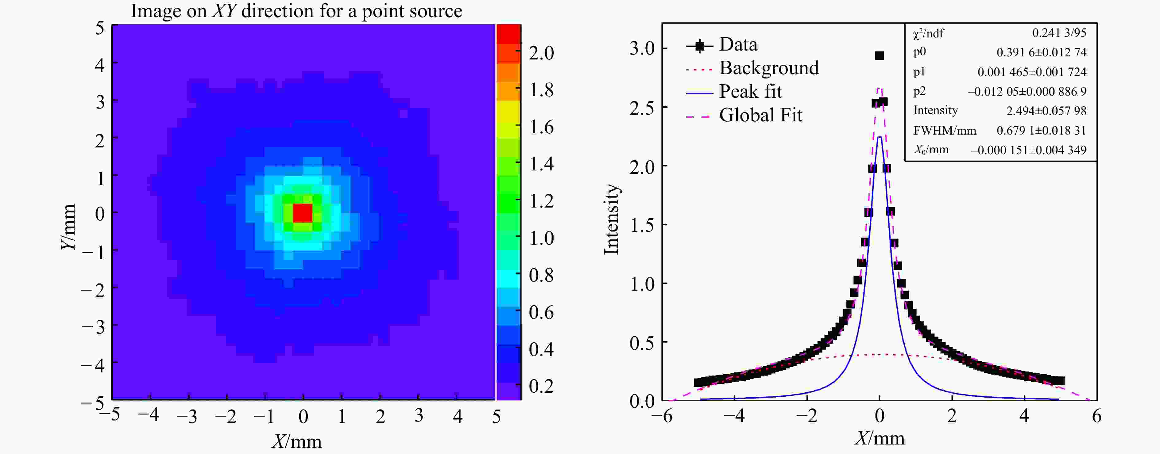
Figure 4. (color online) 2D image of a point-like source reconstruted by back-projection algorithm and the corresponding cross section profile for 150-keV photon scatterred in Silicon.
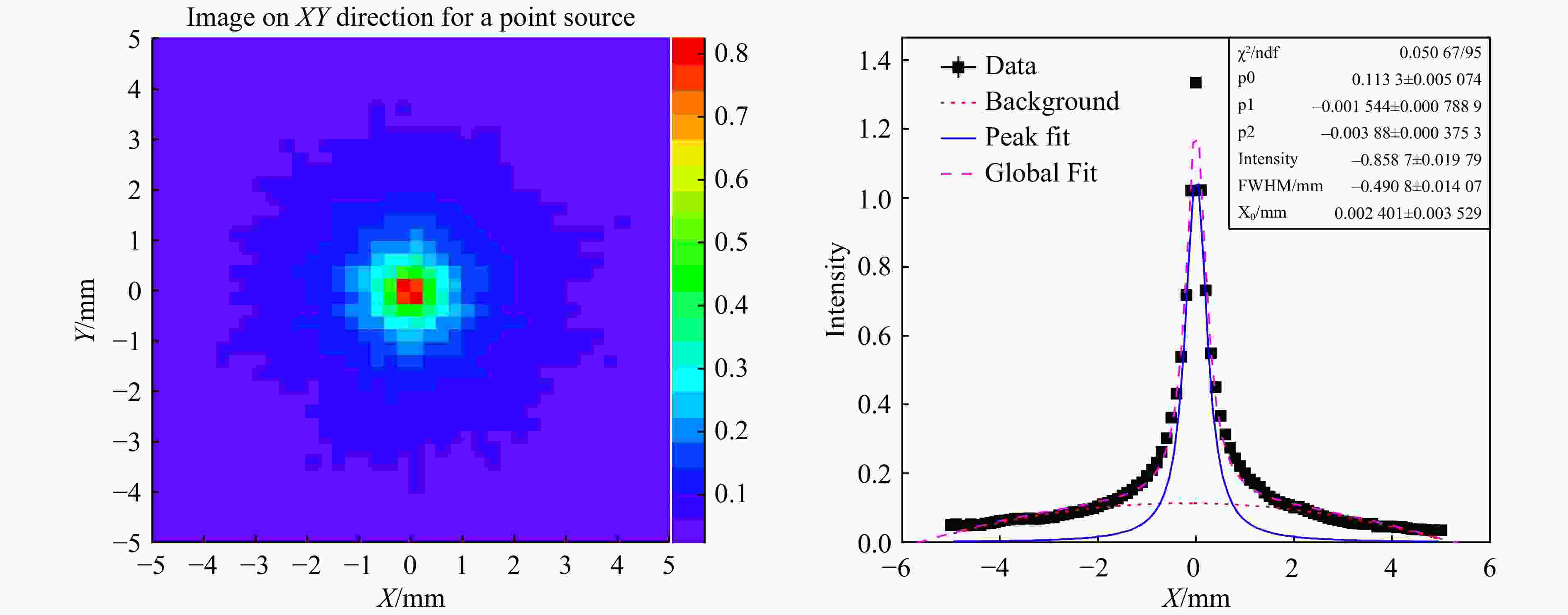
Figure 5. (color online) Same as Fig. 4 but with no Doppler broadening effect.
The FWHMs for the profile of the 2D imaging of a point-like source are summarized in Table 2. As shown, the resolutions for the Compton camera are less than 1.0 mm. It should be noted that only the Doppler broadening effect has been considered here. Table 2 also lists the calculated FWHMs based on Eq. (4) (values in parenthesis). They are in agreement in the order of magnitude with those of the back-projection algorithm. Therefore, Eq. (4) can be used as a tool for approximation of the resolution of Compton camera basing on the ARM.
Table 2. FWHM of cross section profile of 2-D image for different scattering medium (Si, Ge, LSO and BGO) at two incident photon energies (150 and 511 keV).
Energy/keV FWHM of cross section/mm Si Ge BGO LSO 150 0.68 0.82 – – 150 (0.89) (1.20) – – 511 0.50 0.63 0.62 0.61 511 (0.29) (0.44) (0.50) (0.68) -
In present work, the angular resolution measure due to the Doppler broadening effects was simulated by using the Geant4 toolkit employing the G4EMPenelopePhysics model for Silicon, Germanium, LSO and BGO crystals at 150- and 511-keV
$ \gamma $ -rays, respectively. The 2D distribution for the transferred energy versus the scattering angle was also investigated. The simulated results show that better resolution is probable for high-energy$ \gamma $ -rays and, low-Z material is more suited for the candidate for the scattering detector of the Compton Camera. By using the simulated results, the imaging of the gamma source was reconstructed according to the optimized back-projection algorithm. The imaging resolution (FWHM) in this work was overall less than 1.0 mm. For 150-keV$ \gamma $ -rays, FWHMs of 0.68 mm and 0.82 mm were obtained for Silicon and Germanium, respectively and, for 511-keV rays, it was from 0.5 to 0.63 mm for different crystals. Besides, the proposed formula in present work could reproduce the obtained FWHMs.Acknowledgments This work was financially supported by the National Natural Science Foundation of China (NSFC) (11675279, 12075291).
-
摘要: 在重离子癌症治疗中,康普顿相机是一种非常有应用前景的在线监测离子射程的技术。由于康普顿相机使用晶体探测器来确定伽马射线的位置和沉积能量,因此对这些物理量的测量误差会影响康普顿相机的成像分辨率。除了这些测量误差,多普勒展宽效应也会对相机的成像分辨率产生影响。本文使用开源Geant4软件包分别对150和511 keV的伽马射线在几种晶体材料中产生的多普勒展宽效应进行了角分辨模拟。通过对反投影算法的优化和对成像空间中体素的细化,使得康普顿相机的成像分辨率能够达到1.0 mm以上。本工作还基于角分辨标度,推导了一个可快速估计康普顿相机成像分辨率的近似公式。Abstract: In heavy-ion cancer therapy, Compton camera is a promising tool for online monitoring of the range of ions. Compton camera uses crystal detectors to determine the positions and deposited energies of the
$\gamma$ -rays. This will further introduce the errors and affect the actual imaging resolution of the Compton camera, due to the involved Doppler broadening effects influencing the image resolution. This work simulates the angular resolution measure originating from the Doppler broadening effects with Geant4 toolkit for 150 and 511 keV gamma, respectively, in different crystal materials. After optimizing the back-projection algorithm and improving the voxel in imaging interspace, the image resolution can be achieved better than 1.0 mm. An approximate formula is also being proposed to evaluate the image resolution based on the angular resolution measure.-
Key words:
- heavy-ion therapy /
- doppler broadening /
- compton camera /
- Geant4 simulation
-
Figure 1. (color online) Schematic of a Compton camera consisting of a scattering detector and an absorb detector. The scattering angle
$ \theta $ can be constructed by the interaction positions and deposited energies according to the Compton scattering formula.
Figure 2. (color online) Statistical distribution of (a) Doppler broadening, and (b) corresponding ARM.
Figure 3. (color online) 2D histogram of energy-angle distribution for 150-keV gamma in (a) silicon detector and (b) germanium detector, (c) 511-keV gamma in Silicon.
Figure 4. (color online) 2D image of a point-like source reconstruted by back-projection algorithm and the corresponding cross section profile for 150-keV photon scatterred in Silicon.
Table 1. Estimation of FWHM of ARM for different scattering medium (Si, Ge, LSO and BGO) at two incident photon energies (150 and 511 keV).
Energy/keV FWHM of ARM/(°) Si Ge BGO LSO 150 1.7 2.3 – – 511 0.55 0.85 0.95 1.3  下载: 导出CSV
Table 2. FWHM of cross section profile of 2-D image for different scattering medium (Si, Ge, LSO and BGO) at two incident photon energies (150 and 511 keV).
Energy/keV FWHM of cross section/mm Si Ge BGO LSO 150 0.68 0.82 – – 150 (0.89) (1.20) – – 511 0.50 0.63 0.62 0.61 511 (0.29) (0.44) (0.50) (0.68)
下载: 导出CSV
-
[1] ENGHARDT W, CRESPO P, FIEDLER F, et al. Nucl Instr and Meth A, 2004, 525: 284. doi: 10.1016/j.nima.2004.03.128 [2] NISHIO T, OGINO T, NOMURA K, et al. Medical Physics, 2006, 33: 4190. doi: 10.1118/1.2361079 [3] SHAKIRIN G, BRAESS H, FIEDLER F, et al. Physics in Medicine and Biology, 2011, 56: 1281. doi: 10.1088/0031-9155/56/5/004 [4] AMALDI U, HAJDAS W, ILIESCU S, et al. Nucl Instr and Meth A, 2010, 617: 248. doi: 10.1016/j.nima.2009.06.087 [5] HENRIQUET P, TESTA E, CHEVALLIER M, et al. Physics in Medicine and Biology, 2012, 57: 4655. doi: 10.1088/0031-9155/57/14/4655 [6] AGODI C, BATTISTONI G, BELLINI F, et al. Physics in Medicine and Biology, 2012, 57: 5667. doi: 10.1088/0031-9155/57/18/5667 [7] GWOSCH K, HARTMANN B, JAKUBEK J, et al. Physics in Medicine and Biology, 2013, 58: 3755. doi: 10.1088/0031-9155/58/11/3755 [8] TODD R W, NIGHTINGALE J M, EVERETT D B. Nature, 1974, 251: 132. doi: 10.1038/251132a0 [9] KRIMMER J, LEY J L, ABELLAN C, et al. Nucl Instr and Meth A, 2015, 787: 98. doi: 10.1016/j.nima.2014.11.042 [10] PETERSON S W, ROBERTSON D, POLF J. Physics in Medicine and Biology, 2010, 55: 6841. doi: 10.1088/0031-9155/55/22/015 [11] SEO H, PARK J H, USHAKOV A, et al. Journal of Instrumentation, 2011, 6: C01024. doi: 10.1088/1748-0221/6/01/c01024 [12] KUROSAWA S, KUBO H, UENO K, et al. Current Applied Physics, 2012, 12: 364. doi: 10.1016/j.cap.2011.07.027 [13] KORMOLL T, FIEDLER F, SCHOENE S, et al. Nucl Instr and Meth A, 2011, 626: 114. doi: 10.1016/j.nima.2010.10.031 [14] LLOSA G, CABELLO J, CALLIER S, et al. Nucl Instr and Meth A, 2013, 718: 130. doi: 10.1016/j.nima.2012.08.074 [15] MATTAFIRRI S. On Compton Imaging[D]. California: University of California, 2010. [16] HIRASAWA M, TOMITANI T. Physics in Medicine and Biology, 2003, 48: 1009. doi: 10.1109/tns.2003.817951 [17] UCHE C Z, CREE M J, ROUND W H. Australasian Physical and Engineering Sciences in Medicine, 2011, 34: 409. doi: 10.1007/s13246-011-0076-2 [18] CIRRONE G A P, CUTTONE G, DI ROSA F, et al. Nucl Instr and Meth A, 2010, 618: 315. doi: 10.1016/j.nima.2010.02.112 [19] XIAOFENG G, QINGPEI X, DONGFENG T, et al. Applied Radiation and Isotopes, 2017, 124: 93. doi: 10.1016/j.apradiso.2017.03.019 -

 点击查看大图
计量
- 文章访问数: 658
- HTML全文浏览量: 180
- PDF下载量: 44
- 被引次数: 0


 甘公网安备 62010202000723号