


-
In the areas of physics, chemistry, biology, materials, and engineering, a very intense source of neutrons is also very valuable to study the structure and functionality of materials and provide a reference radiation environment. In complement to X-ray or synchrotron sources, neutron sources have several unique advantages[1]. Spallation neutron sources are accelerator-driven facilities to produce high intensity neutrons based on spallation reactions. After successful multi kilowatt spallation neutron sources, several high-power neutron sources are being planned and running, such as SNS[2], J-PARC[3] and ESS[4]. Nonetheless, a high-flux source, which could provide high-energy neutrons and produce rapid irradiation is still missing.
For the engineering of a spallation target, there are many design options such as solid targets, heavy metal fluid targets and rotating solid targets[5]. Recently, the new concept of gravity-driven Dense Granular-flow Target (DGT) was proposed[6]. The movement of the particles make it possible to remove internal deposit heat continuously, while the candidate material has much more choices than traditional liquid targets. This new concept will contribute to the design of a megawatt spallation target for the C-ADS project[7].
The flowing behaviors of particles in DGT is analogous to that of fluids[8] and the deposited high power can be removed and renewed off-line. Moreover, in DGT, heat shock induced by the proton beam is dispersed since granular materials show an excellent buffering performance[9]. Since solid particles are used, it is beneficial to select the materials to reduce corrosion, chemistry-toxicity and radio-toxicity.
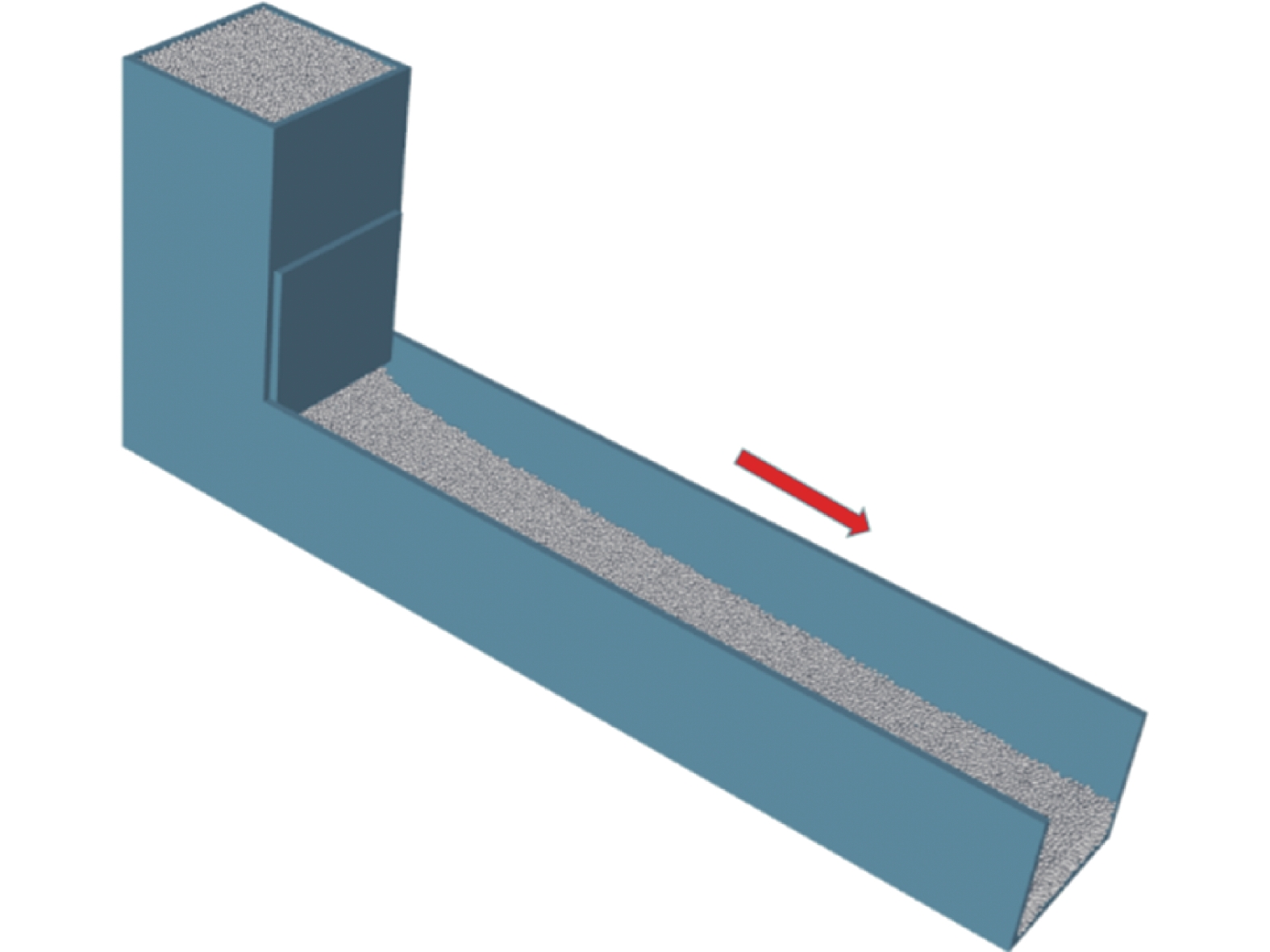
A conceptual design of the gravity-driven chute flow target is schematically shown in Fig. 1[10]. A reservoir or a hopper fills with heavy metal particles acts as a feeder. Downstream there is an inclined chute and the particles discharging from the feeder flow down the chute by gravity. The beam hits the flowing particles at a fixed position. At the end of the chute, the particles flow into a heat exchanger where they are cooled. After filtering, the particles are re-injected into the feeder by a conveying system. The velocity of flow is controlled by adjusting the inclination angles of chute. The chute can be polished to decrease the repose angle. Because the limit of the chute length, the flow is in an accelerating status, which is rarely mentioned in existed literature.
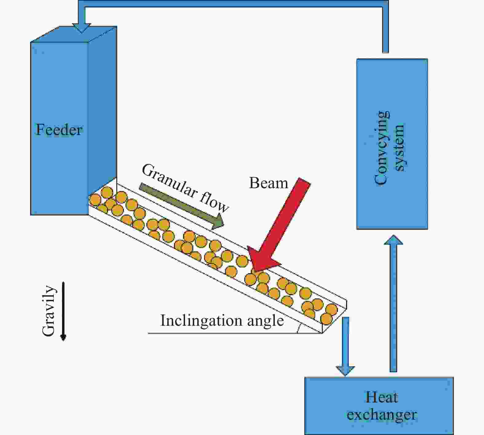
Figure 1. (color online)Schematic diagram of the gravity-driven chute flow target system.
Due to the high heat deposition in the target, it is necessary for investigating that flowability of this flow is acceptable or not. In the past, inclined granular flow was a concern because of the relation with natural phenomenon in nature, such as avalanches and mudslides[11]. The steady, full-developed (SFD) flow was the focus for study of the nature of granular material, especially the difference from the continuum fluids. Whereas surface waves were observed experimentally for both of a rough inclined plate and a flat bottom[12-13], which indicated the unique constitutive relations and more physical quantities, rotation for example, should be included in consideration[14-15].
In this paper, the flowability of the accelerating inclined granular flow was investigated numerically and theoretically. Firstly we performed the simulations to plot the development of the flow and time-averaged flow field in an incline with a finite length. The simulation results were put into stability analysis of Siant-Valent equations. At last a inclined flow with periodic boundary condition was simulation to investigate the responses of interruptions.
-
To simulate the dynamical behaviors of millions of particles, this work was carried out on multiple GPUs by the Discrete Element Method (DEM) code we developed[16-17]. In the DEM model the interactions between the particles are given by Hertz-Mindlin contact model[18-19]. Assuming the particles are identical, the normal and tangential contact forces between two contacting particles are:
$$ \left\{ {\begin{aligned} &{{{{F}}_{i{j_{\rm{n}}}}} = \frac{4}{3}E\sqrt {2r{\delta _{i{j_{\rm{n}}}}}} {{{\delta }}_{i{j_{\rm{n}}}}} - 2\sqrt {\frac{5}{6}} \beta \sqrt {2E\sqrt {\frac{r}{2}{\delta _{i{j_{\rm{n}}}}}} m} {{{v}}_{i{j_{\rm{n}}}}}}\\ &{{{{F}}_{i{j_{\rm t}}}} = 4G\sqrt {2r{\delta _{i{j_{\rm{n}}}}}} {{{\delta }}_{i{j_{\rm{t}}}}} - 2\sqrt {\frac{5}{6}} \kappa \sqrt {2G\sqrt {\frac{r}{2}{\delta _{i{j_{\rm{n}}}}}} m} {{{v}}_{i{j_{\rm{t}}}}}} \end{aligned}} \right., $$ (1) where G is the shear modulus, E is the Young’s Modulus, r is the radius of the particles and m is the mass of particles.
$ {{\delta }}_{{ij}_{\rm{n}}} $ and$ {{\delta }}_{{ij}_{\rm{t}}} $ are normal and tangential displacement vectors, and$ {\delta }_{{ij}_{\rm{n}}} $ and$ {\delta }_{{ij}_{\rm{t}}} $ are their modules, respectively.$ {{v}}_{{ij}_{\rm{n}}} $ and$ {{v}}_{{ij}_{\rm{t}}} $ are normal and tangential relative velocities between the particles I and j.$ \kappa $ is related to the coefficient of restitution. If there is friction, the Coulomb yield criterion |${ F}_{{ij}_{\rm t}} $ | ≤ |μs${ F}_{{ij}_{\rm n}} $ | is satisfied by truncating the magnitude of${ F}_{{ij}_{\rm t}} $ . As a result, if |${ F}_{{ij}_{\rm t}} $ | > μs|${ F}_{{ij}_{\rm n}} $ |,${ F}_{{ij}_{\rm t}} $ =μs|${ F}_{{ij}_{\rm n}} $ |uij/|uij|[19].${ F}_{{ij}_{\rm t}} $ is the friction between two contacting particles i and j, and μs is the friction coefficient.Under gravity field, the equations of motion of the particles are
$$ \left\{ {\begin{split} &{{m_i}{{{a}}_i} = \sum\nolimits_j {\left({{{{F}}_{i{j_{\rm{n}}}}} + {{{F}}_{i{j_{\rm{t}}}}}} \right)} + {m_i}{{g}}}\\ &{{I_i}{{{{\dot \omega }}}_i} = \sum\nolimits_j {\left[ { - \frac{{{r_i}}}{{{r_{ij}}}}{{{r}}_{ij}} \times \left({{{{F}}_{i{j_{\rm{n}}}}} + {{{F}}_{i{j_{\rm{t}}}}}} \right)} \right]} } \end{split}} \right.. $$ (2) These equations are solved by integration using the Velocity-Verlet scheme[20].
-
To simplify the target model, here we investigated the granular flow down an inclined chute discharging through the opening gate. A system, consisting of 1 000 000 mono-disperse beryllium spherical particles (diameter d is 5 mm) was used and the material properties of the reservoir and chute was the same as particles. The walls of the reservoir and chute were smooth and frictional. A Cartesian coordinate system was established: the flow direction was set to x axis and x=0 was at the opening gate; the span-wise direction was set to y axis and y=0 was along the center of the chute; the height (z) direction was perpendicular to the chute and z=0 was at the bottom of the chute. The configuration of the model is schematically shown in Fig. 1 and the material parameters are presented in Table 1. The time-step in DEM simulations was 5×10⁻⁷ s. Initially a random filling process was used to fill the reservoir with the particles until reach a static packing. Then the gate was opened and steady state flow was allowed to develop before acquiring the data used for subsequent analysis.
Table 1. Geometrical and material parameters.
Quantity Symbol/Unit Value Diameter of particles d/mm 5 Width of the chute W/mm 40d Length of the chute L/mm 600d Height of the gate G/mm 25d Inclination angle of the chute θc/(°) 25° Length/width of the reservoir D/mm 40d Elastic modulus E/GPa 287 Poisson’s ratio ν 0.032 Particle-particle and particle-wall friction coefficients μ 0.2 Density ρ/(kg/m3) 1 850 Particle-particle and particle-wall coefficient of restitution ε 0.9 Hardness H/GPa 1.67 -
Here we use granular flows down inclined flat planes, with periodic boundaries in the x (flow) and y (span-wise) directions, to study the stability of the inclined flows. A system, consisting of 10 000 mono-disperse beryllium spherical particles (diameter d is 5 mm) was used. A Cartesian coordinate system was established: the flow direction was set to x axis and x=0 was at the center of the length; the span-wise direction was set to y axis and y=0 was along the center of the chute; the height (z) direction was perpendicular to the chute and z=0 was at the bottom of the chute. The parameters of material properties are also shown in Table 1. The time-step in DEM simulations was 5×10⁻⁷ s too. The simulation cell dimensions in the x and y direction were 20d and 20d respectively, resulting in an approximately 25d height in the z direction. Initially, 10 000 particles randomly dropped under gravity into the horizontal plane and a static packing was achieved after a while. Then the system was tilted to a desired inclination angle (25°) to initiate the flow. At this inclined Angle the granular flow will be accelerative. After reaching a steady flows, perturbation was added to test the stability of the flows and then Lyapunov exponent
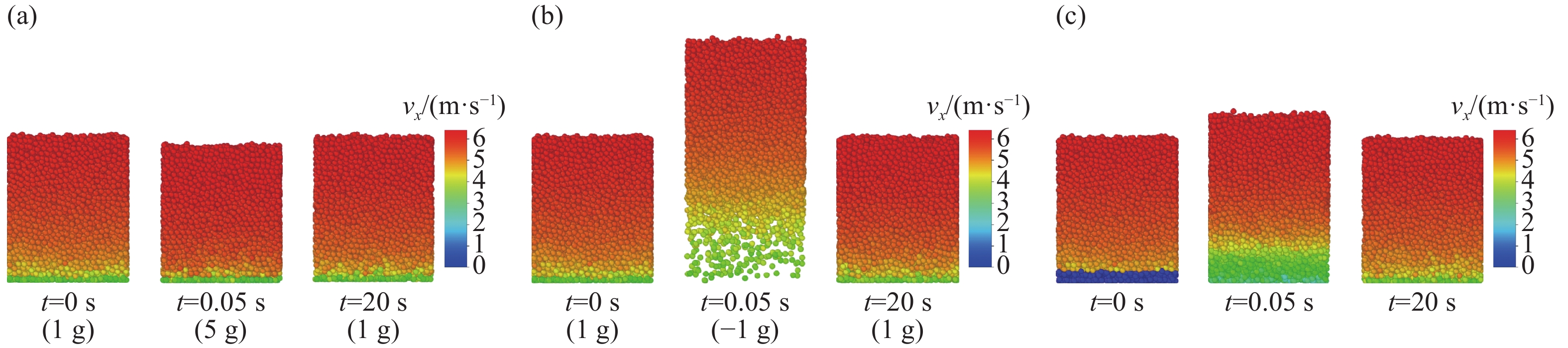
$ \xi $ was calculated by fitting the formula:$\Delta E\left(t \right) = \Delta E\left(0 \right){\rm{exp}}\left({ - \xi t} \right)$ , where$ \Delta E $ is the absolute average difference of per particle between the perturbed system and the control no-perturbed system. In our study, three perturbation protocols (Fig. 2) were considered: (a) changing the gravity from 1 g to 5 g during t=0~0.1 s; (b) changing the gravity from 1 to –1 g during t=0~0.1 s; (c) pining the bottom particles instantaneously at t=0 s.
Figure 2. (color online)The snapshots of system with three perturbation protocols.
-
In the process, Voronoi volume of each particle was calculated and the local volume fraction was ratio of particle volume and its Voronoi volume. Then these local volume fractions were aligned as property of the corresponding particle and it was time-averaged by the same procedure of the particle velocity[21]. In the procedure, hundreds of snapshots were gathered and the space of each snapshot was divided into the same meshes. The particle quantities (including velocity, volume fractions and etc.) of each mesh were averaged by the appearance time of particles within this mesh to obtain the time-averaged quantities.
The virial stress is commonly used to find the macroscopic (continuum) stress in molecular dynamics systems, and is defined as
$$\begin{split} {\sigma _{ij}} = & \frac{1}{V}\mathop \sum \limits_{k \in V} \left[ - {m^{\left(k \right)}}\left({u_i^{\left(k \right)} - \overline {{u_i}} } \right)\left({u_j^{\left(k \right)} - {{\bar u}_j}} \right)\right. +\\ &\left. \frac{1}{2}\mathop \sum \limits_{l \in V} \left({x_i^{\left(l \right)} - x_i^{\left(k \right)}} \right)f_j^{\left({kl} \right)} \right], \end{split}$$ (3) where
$ k $ and$ l $ are atoms in the domain,$ V $ is the volume of the domain,$ {m}^{\left(k\right)} $ is the mass of atom$ k $ ,$ {{u}_{i}}^{\left(k\right)} $ is the$ {i}^{th} $ component of the velocity of atom$ k $ ,$ {\bar{u}}_{j} $ is the$ {j}^{th} $ component of the average velocity of atoms in the volume,$ {x}_{i}^{\left(k\right)} $ is the$ {i}^{th} $ component of the position of atom$ k $ , and$ {f}_{i}^{\left(kl\right)} $ is the$ {i}^{th} $ component of the force applied on atom$ k $ by atom$ l $ . In this paper, the time-series profiles of particle positions and velocities were collected and space in the chute was divided into subdomain to calculate the time-averaged virial stresses. -
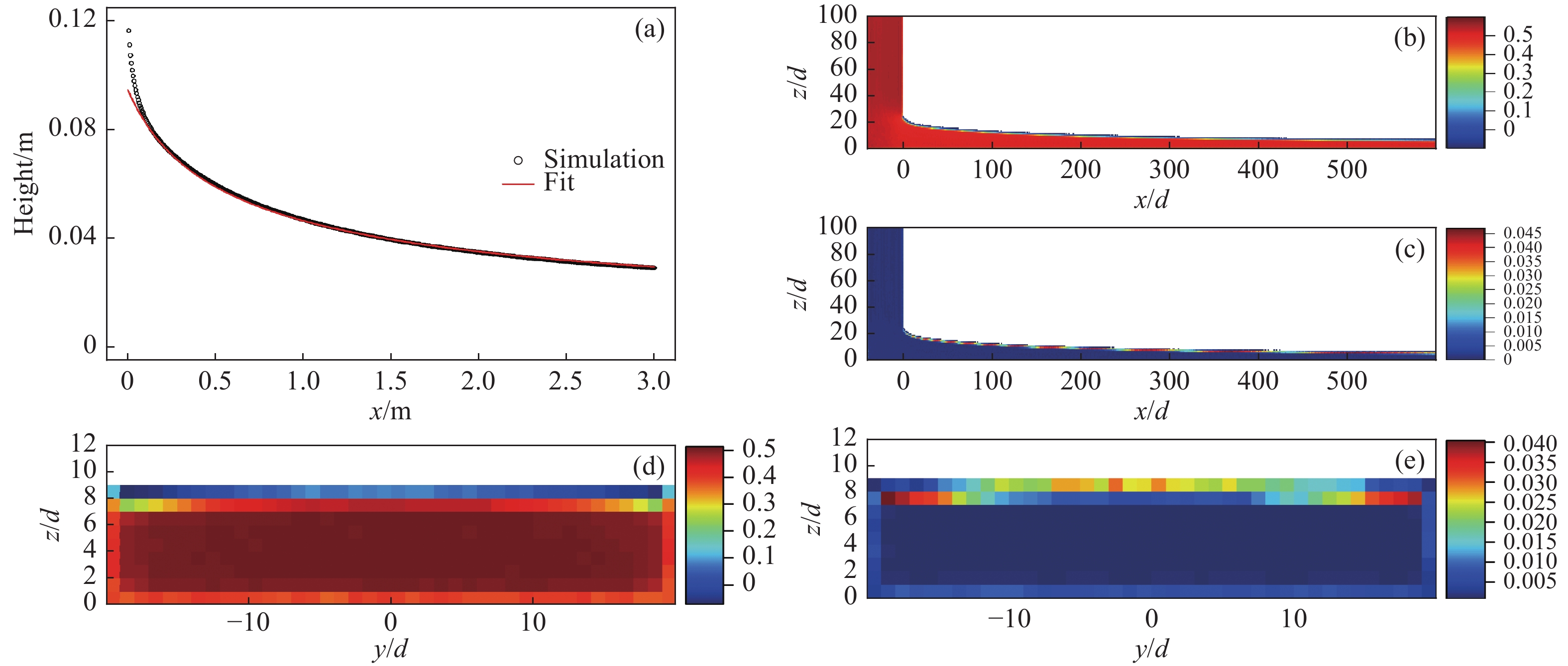
In an inclined chute with a rough base, the particles behave like solid, fluid or gas by varying the inclination angles[22-23]. If the base is sufficiently smooth, the flow is simple and adjustable. To simplify the model, monosize-distribution tungsten particles (diameter d is 5 mm) were simulated. The material of the reservoir and chute was the same as particles and their roughness was assumed as nil. The configuration of the ‘the basic’ case is schematically shown in Fig. 3. The geometrical and material parameters in the basic case are shown in Table 1. The time-step in DEM simulations was 5×10⁻⁷ s too. The inclination angle was set to 25° to avoid potential stagnant or gaseous state in the downstream chute[23]. Initially the particles were packed in the reservoir and then were discharged through an opening gate. After 20 s later, the time-averaged velocity and volume fraction fields along the chute flow were plotted and the stability of the flow was analyzed.

Figure 3. (color online)Configuration of the simple model of chute flows. The red arrow denotes the flowing direction.
The morphology of the flow was nearly stable over time [see in Fig. 4(a)]. From the gate to x=600d, fluctuation of the height of the accelerating flow was less than 10% which was consistent with Holyoake et al[24]’s results (see in appendix for detailed analysis of the fluctuation and stability).
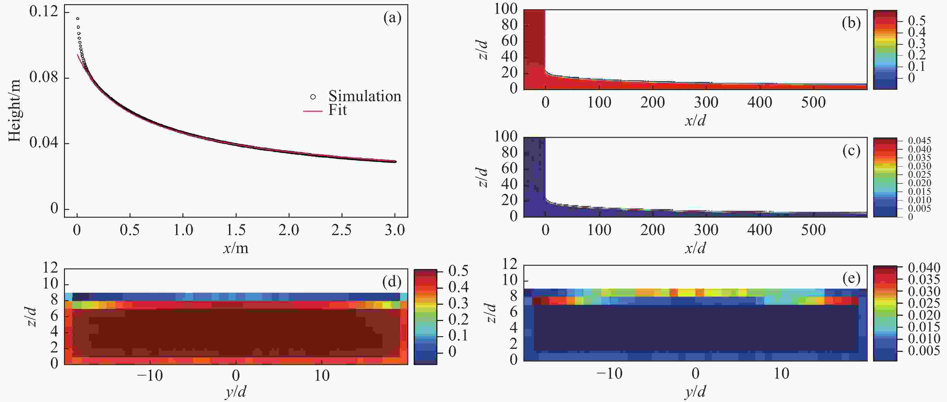
Figure 4. (color online)The simulation results of granular flows in a chute with gate height of 25d, chute width of 40d and inclination angle of 25°.
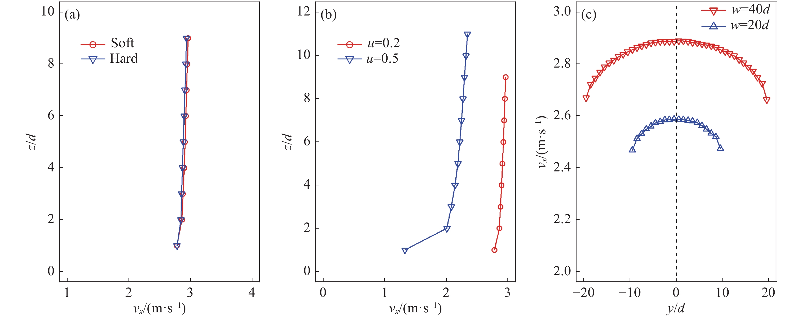
The time-averaged velocity and volume fraction fields are shown in Fig. 4(b) and 4(c), where the volume fraction fields were calculated by plotting the Voronoi diagrams[25]. The volume fraction in the chute flow varied from 0.5 to 0.6 except at the free surface and bottom, which was consistent with the volume fraction in random packing. Fig. 4(d) shows the influence of the walls on the volume fraction. Similar to the bottom, the volume fraction near the walls varied between 0.4 and 0.5. From the spatial profiles of
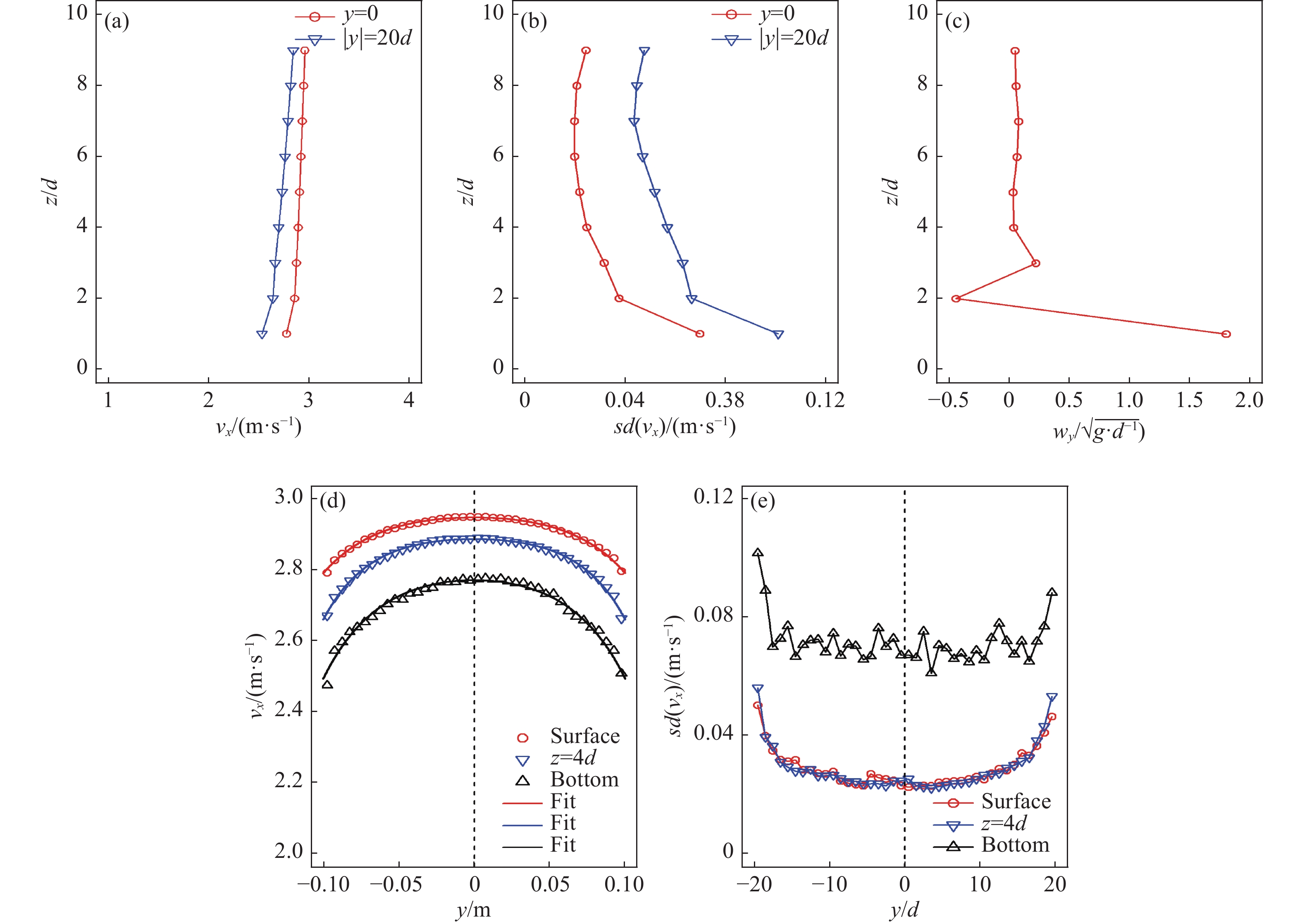
$ {v}_{x} $ , it appeared that there is nearly a plug flow in the chute as the variation of$ {v}_{x} $ is small along the depth. The influence of the walls on$ {v}_{x} $ is shown in Fig. 5(d) and it was found that central particles move more quickly than particles near the sidewalls (the discrepancy is less than 10%).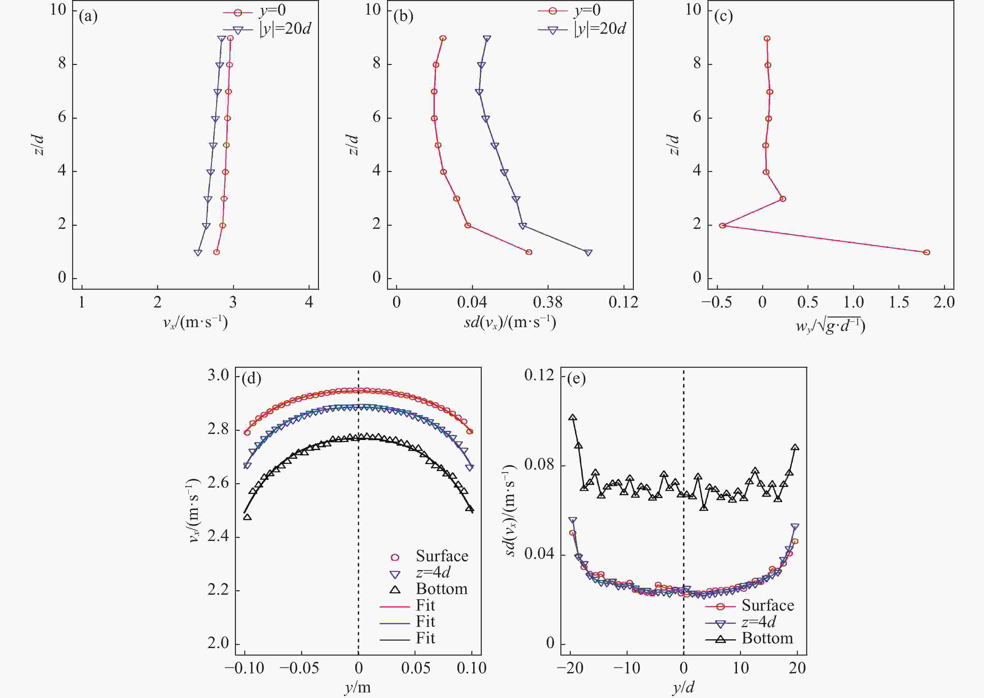
Figure 5. (color online)Spatial profile of the simulation results with gate height of 25d, chute width of 40d and inclination angle of 25°.
From former studies, it showed there is a basal rolling layer in a stable, fully developed flow on the flat, frictional incline[26], which was also observed in this accelerating flow [see in Fig. 5(c)]. Interestingly, the result showed that the wy of second layer is opposite, which agrees with the previous picture[27]. The profile of width-averaged and depth-averaged vx could be fitted by using the following function:
$$\overline {{v_x}} \left(x \right) = \sqrt {{v_0}^2 + \frac{\beta }{\gamma }\big[ {1 - {\rm{exp}}\left({ - \gamma x} \right)} \big]} ,$$ (4) in Ref. [24], fitting parameters
$ {v}_{0}=1.191\;{\rm{m}}/{\rm{s}} $ ,$ \beta =4.488\;{\rm{m}}/{{\rm{s}}}^{2} $ ,$ \gamma =0.024\;{{\rm{m}}}^{-1} $ , which implied that vx will converge to 13.7 m/s when$ x\to \infty $ . The height h(x) could also be fitted if the flux conversation was assumed in the accelerating flow:$$h\left(x \right) = {C_0}/\overline {{v_x}} \left(x \right).$$ (5) Here the fitting parameter
$ {C}_{0}=0.113\;{{\rm{m}}}^{2}/{\rm{s}} $ and fitting result is shown in Fig. 4(a). The influence of sidewalls on the velocity profile could be evaluated by using fitting formula in Ref. [28]:$${v_x}\left({x,y,z} \right) = {\rm{\alpha }}\left({x,z} \right) - {{B}}\left({x,z} \right){\rm{cosh}}\left({ - y/\varLambda } \right).$$ (6) It is noted that this formula is used for studying about the influence of sidewalls on the surface velocity in granular avalanche[28] but it is also available for inner and bottom velocities here [see in Fig. 5(d)]. The fitting parameter
$ \varLambda =0.037\;{\rm{m}} $ here and was an invariant. To evaluate the stability of the flow, the temporal profiles of velocity and volume fraction fields were analyzed and their standard error was calculated. Here it was showed that the standard errors of volume fraction are very small except at the free surface. For$ {v}_{x} $ , the standard error on the bottom was more than the standard error at the free surface and both were relatively small.To study the inferences of material parameters on the chute flows, comparing simulations were performed and the results are shown in Fig. 6 and Table 2. It appeared that the friction coefficient and chute width influence the flows. The flow rate was bigger when the particles had a low modulus of elasticity (E=5×10⁶ Pa), which was consistent with previous observation in hopper flow[29]. Moreover, the flow was slower in the narrower chute.
Table 2. The influences of material and geometrical parameters on the mass flow rate.
Case Mass flow rate/(kg/s) Basic case 26.8 Softer particles (E=5×10⁶ Pa) 29.3 Higher friction coefficient (μ=0.5) 18.8 Narrower chute (W=10 cm) 10.6 Bigger particles (d=10 mm) 25.6 Higher density of particles (ρ=7 800 kg/m3) 120.4 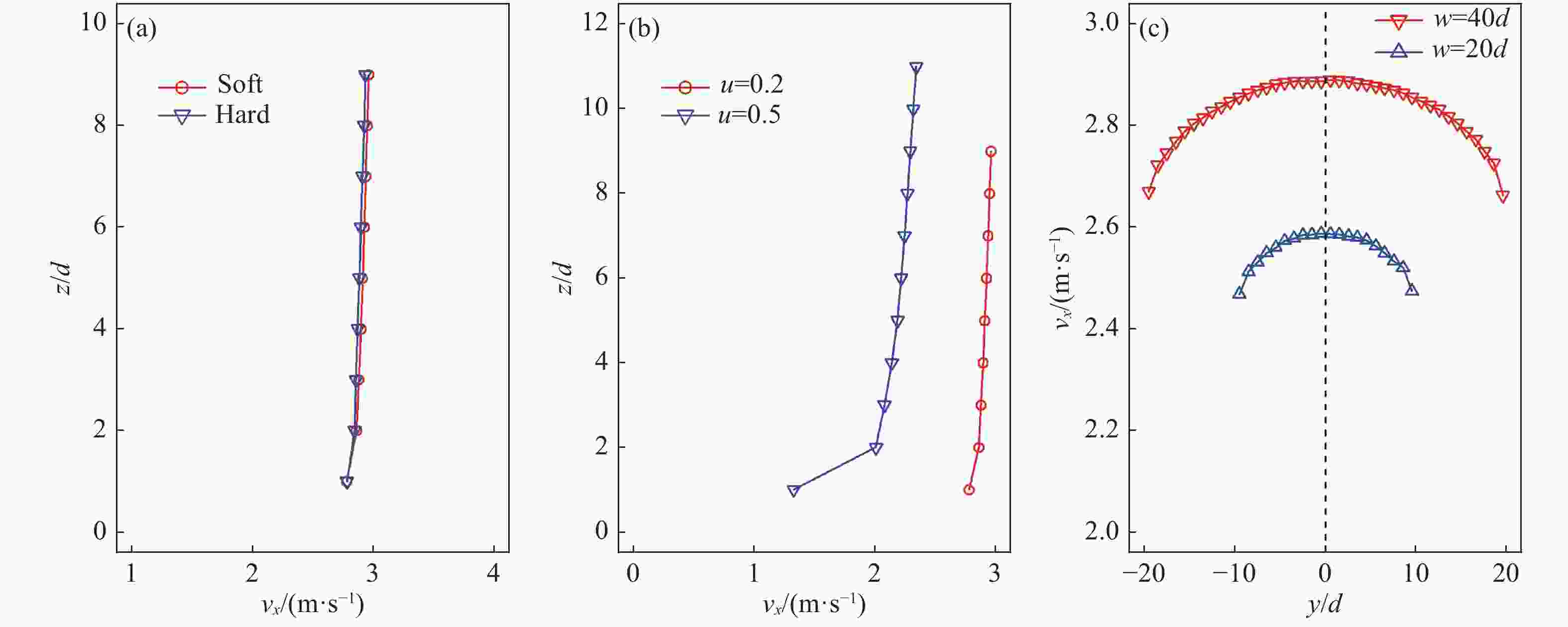
Figure 6. (color online)Spatial profile of
$ {v}_{x} $ at different depths at x=300d. A comparison between (a) hard and soft particles; (b) different frictional coefficients; (c) different chute widths. -
To study the stability of the flow, here we used the linear stability analysis developed in Forterre and Pouliquen’s paper[12]. The difference here was that an accelerating flow, instead of a steady uniform flow, is analyzed. The Saint-Valent equations are used to describe the dynamics of the inclined flow:
$$\frac{{\partial h}}{{\partial t}} + \frac{{\partial h\overline {{v_x}} }}{{\partial x}} = 0,$$ (7) $$\rho \left( {\frac{{\partial h\overline {{v_x}} }}{{\partial t}} \!\!+\!\! \alpha \frac{{\partial h{{\overline {{v_x}} }^2}}}{{\partial x}}} \right) \!\!=\!\! \left( {{\rm{tan}}\theta \!\!- \!\!{\mu _{{\rm{eff}}}}\left( {\overline {{v_x}} ,h} \right) \!\!-\!\! K\frac{{\partial h}}{{\partial x}}} \right)\rho gh{\rm{cos}}\theta .$$ (8) In the steady accelerating flow, the spatial profiles of
$\overline {{v_{{x}}}} \left( x \right)$ and h(x) are described by Eq. (4) and Eq. (5). The coefficient$ \alpha $ is related to the assumed velocity profile across the layer. The coefficient K represents the ratio of the normal stress in x-direction to the normal stress in z-direction and K=1 is assumed here[12]. The dimensionless equations are as follows:$$\frac{{\partial \tilde h}}{{\partial \tau }} + \frac{{\partial \tilde h\tilde u}}{{\partial {\rm{\chi }}}} = 0,$$ (9) $${F_0}^2\left( {\frac{{\partial \tilde h\tilde u}}{{\partial \tau }} + \alpha \frac{{\partial \tilde h{{\tilde u}^2}}}{{\partial {\rm{\chi }}}}} \right) = \left( {{\rm{tan}}\theta - {\mu _{{\rm{eff}}}}\left( {\tilde u,\tilde h} \right) - \frac{{\partial \tilde h}}{{\partial {\rm{\chi }}}}} \right)\tilde h.$$ (10) The dimensionless variables are given by
$\tilde u = \overline {{v_x}} /{v_0} = \sqrt {1 + \eta \left( {1 - {{\rm e}^{ - \delta \chi }}} \right)} $ ,$\tilde h = \frac{h}{{{C_0}/{v_0}}} = 1/\tilde u$ ,${\rm{\chi }} = \frac{x}{{{C_0}/{v_0}}}$ ,$ \tau =\frac{{{v}_{0}}^{2}}{{C}_{0}}t $ ,$\eta = \beta /\gamma {v_0}^2$ ,$ \delta =\frac{\gamma {C}_{0}}{{v}_{0}} $ ,$ {F}_{0}=\frac{{v}_{0}}{\sqrt{g{C}_{0}/{v}_{0}{\cos}\theta }} $ .Suppose there is a perturbation in this flow:
$u'\left( {\chi ,\tau } \right) = \tilde u\left( {\chi ,\tau } \right) + \hat u{{\rm{e}}^{{\rm{i}}\left( {k\chi - \omega \tau } \right)}}$ ,$h'\left( {\chi ,\tau } \right) = \tilde h\left( {\chi ,\tau } \right) + \hat h{{\rm{e}}^{{\rm{i}}\left( {k\chi - \omega \tau } \right)}}$ ($\hat u \ll 1,\hat h \ll 1$ ), and${\mu _{{\rm{eff}}}}$ can be expressed with first-order expansion:${\mu _{{\rm{eff}}}}\left( {\tilde u,\tilde h} \right) = {\mu _0} + a\frac{{\partial {\mu _{{\rm{eff}}}}}}{{\partial \tilde u}} + b\frac{{\partial {\mu _{{\rm{eff}}}}}}{{\partial \tilde h}}$ . The dispersion relation can be obtained by substituting expression of$\tilde u,\tilde h,{\mu _{{\rm{eff}}}}$ into Eq. (9), Eq. (10):$$\begin{aligned} &\tan \theta \frac{{\partial \tilde h}}{{\partial \chi }}\! -\! {\left( {\frac{{\partial \tilde h}}{{\partial \chi }}} \right)^2}\! + \!{k^2}{{\tilde h}^2} \!- \!{\mu _0}\frac{{\partial \tilde h}}{{\partial \chi }} \!+\! {\rm{i}}k\tan \theta \tilde h\!-\! {\rm{}}{F_0}^2{\omega ^2}\tilde h -\\& b\frac{{\partial \tilde h}}{{\partial \chi }}\tilde h - 2{\rm{i}}k\frac{{\partial \tilde h}}{{\partial \chi }}\tilde h + {\rm{}}a\frac{{\partial \tilde u}}{{\partial \chi }}\tilde h - {\rm{i}}a\omega \tilde h{\rm{}} - {\rm{i}}k{\mu _{{\rm{eff}}}}\tilde h - {\rm{i}}bk{{\tilde h}^2} +\\ & {\rm{i}}{F_0}^2\omega \frac{{\partial \tilde h}}{{\partial \chi }}\tilde u - {\rm{i}}{F_0}^2\omega \frac{{\partial \tilde u}}{{\partial \chi }}\tilde h + 2{F_0}^2{\rm{\alpha }}{\left( {\frac{{\partial \tilde u}}{{\partial \chi }}} \right)^2}\tilde h + {\rm{i}}ak\tilde h\tilde u -\\ & {F_0}^2{\rm{\alpha }}{k^2}\tilde h{{\tilde u}^2} - 2{\rm{i}}{F_0}^2{\rm{\alpha }}\omega \frac{{\partial \tilde h}}{{\partial \chi }}\tilde u - 2{\rm{i}}{F_0}^2{\rm{\alpha }}\omega \frac{{\partial \tilde u}}{{\partial \chi }}\tilde h{\rm{}} +\\ & {\rm{i}}{F_0}^2{\rm{\alpha }}k\frac{{\partial \tilde h}}{{\partial \chi }}{{\tilde u}^2} + 2{\rm{i}}{F_0}^2{\rm{\alpha }}k{\rm{}}\frac{{\partial \tilde u}}{{\partial \chi }}\tilde h\tilde u +\\ & 2{F_0}^2{\rm{\alpha }}k\omega \tilde h\tilde u = 0.\\[-15pt] \end{aligned}$$ (11) The pulsation ω is real and the wavenumber k is complex:
$ k={k}_{r}+{\rm{i}}{k}_{i} $ , then we have$${k_r}^{1,2} = - \frac{{{a_{12}}}}{{2{a_2}}} \pm \frac{{\sqrt 2 {b_1}}}{{\sqrt { - {b_2} + \sqrt {b_2^2 + 4b_1^2} } }},$$ (12) $${k_i}^{1,2} = - \frac{{{a_{11}}}}{{2{a_2}}} \pm \sqrt {\frac{{ - {b_2} + \sqrt {b_2^2 + 4b_1^2} }}{2}} ,$$ (13) where
$$ {b}_{1}=\dfrac{{a}_{11}{a}_{12}}{4{a}_{2}^{2}}-\dfrac{{a}_{01}}{2{a}_{2}}$$ $$ {b}_{2}=\frac{{a}_{12}^{2}}{4{a}_{2}^{2}}-\frac{{a}_{11}^{2}}{4{a}_{2}^{2}}-\frac{{a}_{02}}{{a}_{2}}{,} $$ $${a_2} = {\tilde h^2} - {F_0}^2{\rm{\alpha }}\tilde h{\tilde u^2}{\rm{}},$$ $$\begin{split} {a}_{11}=&\tilde {h}{\tan}\theta -{\mu }_{0}\tilde {h}-b{\tilde {h}}^{2}-2\tilde {h}\frac{\partial \tilde {h}}{\partial \chi }+a\tilde {h}\tilde {u}+\\&{{F}_{0}}^{2}{\rm{\alpha }}\frac{\partial \tilde {h}}{\partial \chi }{u}^{2}+2{{F}_{0}}^{2}{\rm{\alpha }}\tilde {h}\tilde {u}\frac{\partial \tilde {u}}{\partial \chi }{,} \end{split}$$ $$ {a}_{12}=2{{F}_{0}}^{2}{\rm{\alpha }}\omega \tilde {h}\tilde {u}{,} $$ $$\begin{split} {a}_{01}=& {{F}_{0}}^{2}\omega \frac{\partial \tilde {h}}{\partial \chi }\tilde {u}-{{F}_{0}}^{2}\omega \tilde {h}\frac{\partial \tilde {u}}{\partial \chi }-a\omega \tilde {h}-\\&2{{F}_{0}}^{2}{\rm{\alpha }}\omega \tilde {h}\frac{\partial \tilde {u}}{\partial \chi }-\;2{{F}_{0}}^{2}{\rm{\alpha }}\omega \frac{\partial \tilde {h}}{\partial \chi }\tilde {u}{,} \end{split}$$ $$\begin{split} {a}_{02}=&\frac{\partial \tilde {h}}{\partial \chi }{\tan}\theta -{\mu }_{0}\frac{\partial \tilde {h}}{\partial \chi }-{\left(\frac{\partial \tilde {h}}{\partial \chi }\right)}^{2}-{{F}_{0}}^{2}{\omega }^{2}\tilde {h}-\\&bh\frac{\partial \tilde {h}}{\partial \chi }+a\tilde {h}\frac{\partial \tilde {u}}{\partial \chi }+2{{F}_{0}}^{2}{\rm{\alpha }}\tilde {h}{\left(\frac{\partial \tilde {u}}{\partial \chi }\right)}^{2}{.} \end{split}$$ The expression of friction coefficient can be obtained by substituting expression of
$ \tilde {u} $ into Eq. (10).$$ {\mu }_{\rm{eff}}={\tan}\theta +\frac{1}{{\tilde {u}}^{2}}\frac{\partial \tilde {u}}{\partial \chi }-{{F}_{0}}^{2}\alpha \tilde {u}\frac{\partial \tilde {u}}{\partial \chi }{.} $$ (14) We can analyze
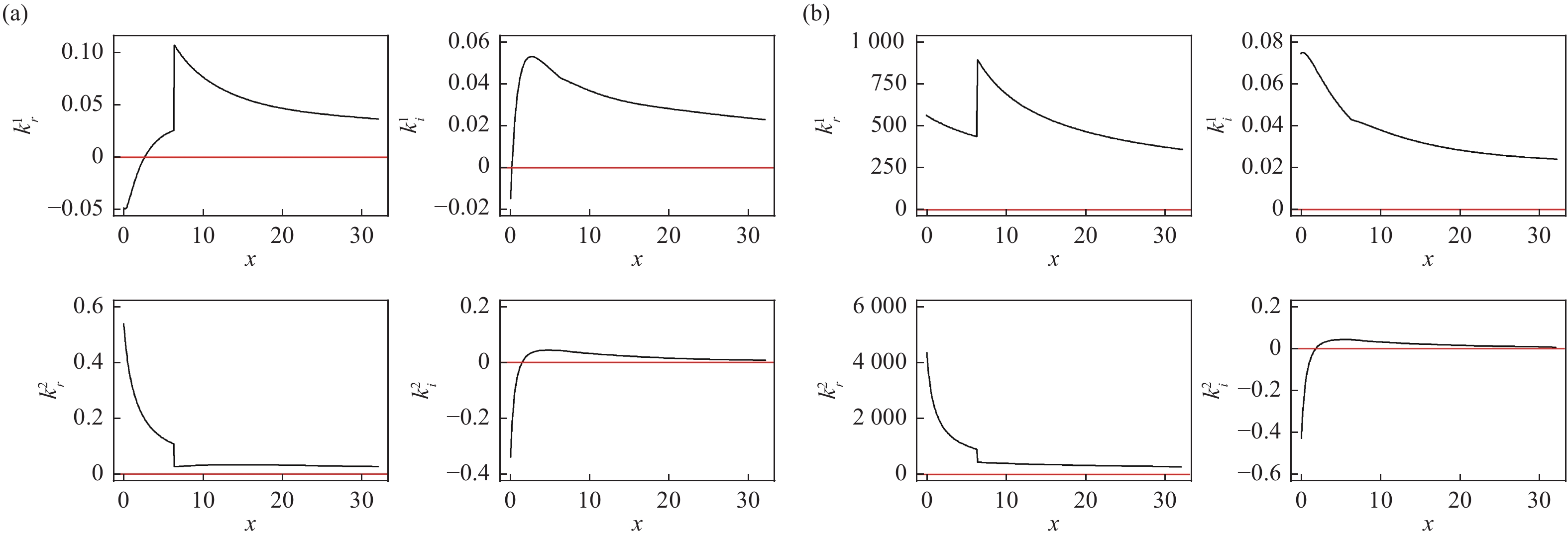
$ {{k}_{r}}^{{1,2}},{{k}_{i}}^{{1,2}} $ in our simulation case by substituting the fitting results of Eq. (4) and Eq. (5) into Eq. (12), Eq. (13) and using Eq. (14). Here$ \alpha $ was assumed to be 1 because the flow is nearly a plug flow. The numerical solutions of$ {{k}_{r}}^{{1,2}},{{k}_{i}}^{{1,2}} $ are plotted in Fig. 7 when the frequency is very low ($ \omega $ =0.1 Hz) or very high ($ \omega $ =1 000 Hz)[12]. It was found both of$ {{k}_{i}}^{{1,2}} $ are positive in the chute (0<x<3 m) except near the outlet, which indicated that the flow is stable here.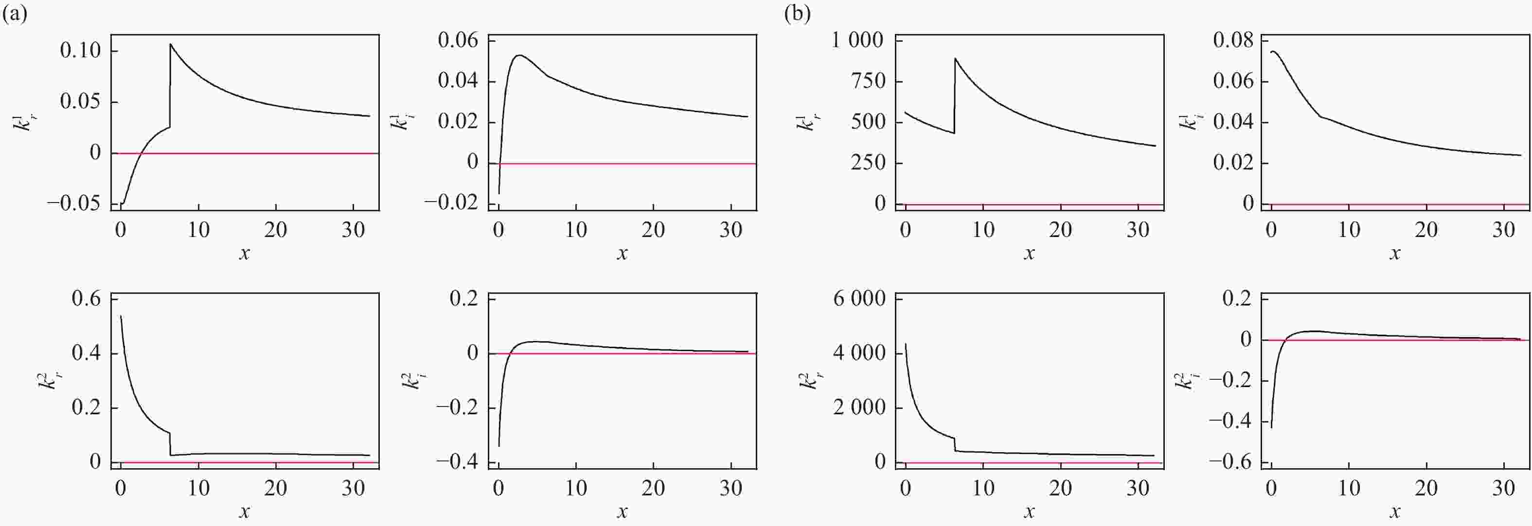
Figure 7. (color online)
$ {{k}_{r}}^{{1,2}},{{k}_{i}}^{{1,2}} $ vs$ \chi $ when$ \omega $ =0.1 Hz (a) and 1 000 Hz (b).The
$ {\mu }_{\rm{eff}}\left(x\right) $ could also be obtained by directly computing the spatial profiles of viral stress and to calculate$ {\mu }_{\rm{eff}}=\left|\frac{{\sigma }_{zx}}{{\sigma }_{zz}}\right| $ . Fig. 8 shows that there is a little discrepancy between$ {\mu }_{\rm{eff}}\left(x\right) $ calculated from the stress profiles and$ {\mu }_{\rm{eff}}\left(x\right) $ calculated from Eq. (14). It might result from the influences of sidewalls.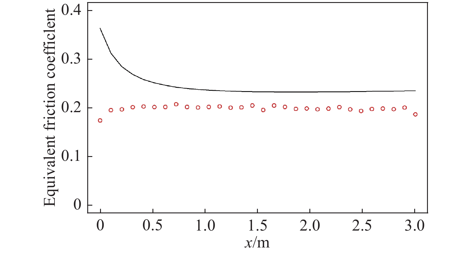
Figure 8. (color online)The
$ {\mu }_{\rm{eff}}\left(x\right) $ calculated from stress profiles and from Eq. (14). -
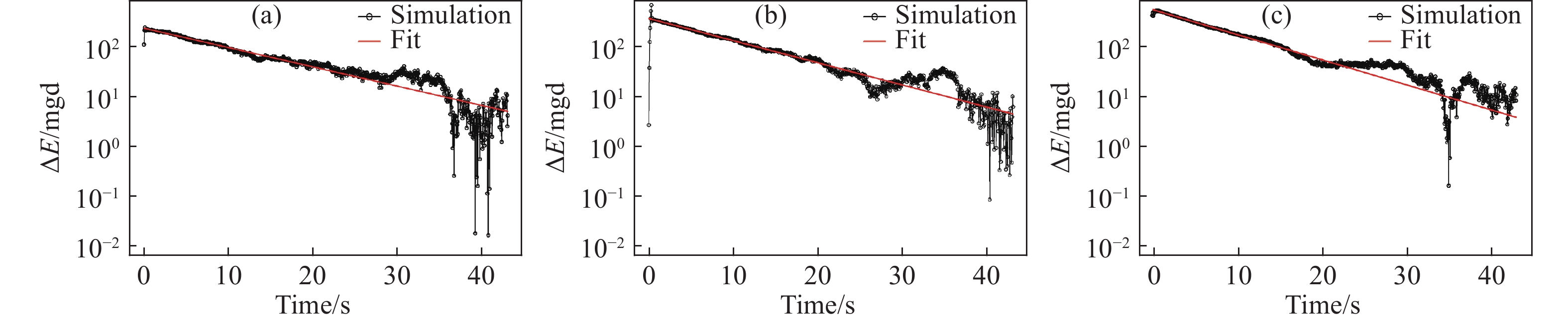
To study the stability of a steady inclined flows, a steady granular flows with a periodic boundary condition was simulated[30] and was perturbed to calculate the Lyapunov exponent. The perturbation protocols are introduced in Fig. 7.
A fitting formula was used to calculate the Lyapunov exponent:
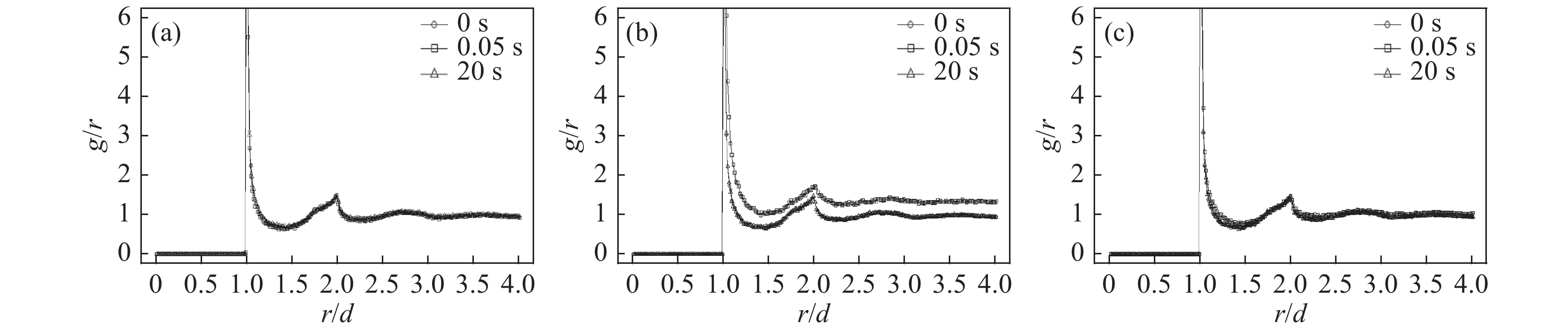
$ \Delta E\left({{t}}\right)=\Delta E\left(0\right)\exp (-\xi t) $ . In all these three cases, the Lyapunov exponent was approximately –0.1, which indicated that the system has an intrinsic stability mechanism (see in Fig. 9). The influence on the radial distribution of this system would also be reduced over time (Fig. 10).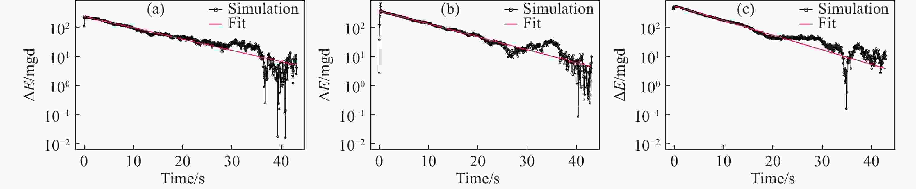
Figure 9. (color online)The variations of system energy in three cases: (a) changing the gravity from 1 to 5 g for 0.1 s; (b) changing the gravity from 1 to –1 g for 0.1 s; (c) pining the bottom particles instantaneously.
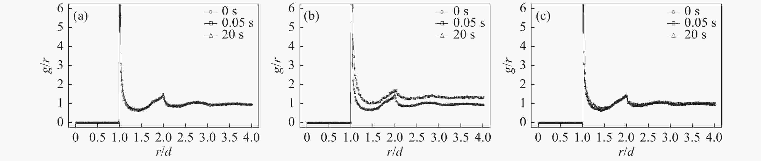
Figure 10. The variations of radial distribution in these three cases.
-
Here the flowability of an accelerating inclined dense granular flow was investigated by simulations. It was found that in this accelerating flow there were slight fluctuations of velocity and density and no surface wave was observed. Furthermore, the stability of the flow was studied by using linear stability analysis and calculating Lyapunov exponent. All the results demonstrated the constancy and stability of the accelerating flow and supported the availability of this flow to be a proposal design of high-power target. Furthur work will focus on the development of simulation model for a better accrodance with the experimental conditions.
Acknowledgment Project supported by the National Natural Science Foundation of China (11474326), Young Scholar of CAS "Light of West China" Program (29Y922030) and the Strategic Priority Research Program of Chinese Academy of Sciences (XDA21010202).
-
摘要: 研究了中子辐照装置密集斜槽流颗粒靶设计的流动性,该靶设计能够提供适用于聚变反应堆材料研究的高能中子。本文通过数值模拟和理论分析的方法描述了流动的稳定性和稳固性,这在其他文献中很少被提及。结果发现,25°对于稳定的流动是可以接受的,这种颗粒流有潜力成为热介质的选择。
-
关键词:
- dense granular target /
- inclined flow /
- stability /
- constancy /
- DEM simulation
Abstract: This paper presented a study of flowability of the inclined dense granular-flow target for a neutron irradiation facility, which is capable of providing high-energy neutrons suitable to advance fusion reactor material research. The results from simulations and theoretical analysis described the constancy and stability of the flow, which was rarely mentioned before. It was found that 25° was acceptable for a steady and stable accelerating flow and all the results supported the availability of this granular flow for a potential choice of the heat medium.-
Key words:
- dense granular target /
- inclined flow /
- stability /
- constancy /
- DEM simulation
-
Figure 1. (color online)Schematic diagram of the gravity-driven chute flow target system.
Figure 2. (color online)The snapshots of system with three perturbation protocols.
(a) changing the gravity from 1 to 5 g during t=0~0.1 s; (b) changing the gravity from 1 g to –1 g during t=0~0.1 s; (c) pining the bottom particles instantaneously at t=0 s. The color scale indicates the velocity magnitude in x direction.
Figure 3. (color online)Configuration of the simple model of chute flows. The red arrow denotes the flowing direction.
Figure 4. (color online)The simulation results of granular flows in a chute with gate height of 25d, chute width of 40d and inclination angle of 25°.
(a) The variation of the shape of the flow. (b) Spatial profile of volume fraction in the central cross section along x direction. (c) Spatial profile of standard deviation of volume fraction in the central cross section along x direction. (d) Spatial profile of volume fraction in the cross section which is perpendicular to x direction at x=300d. (e) Spatial profile of standard deviation of volume fraction in the cross section which is perpendicular to x direction at x=300d.
Figure 5. (color online)Spatial profile of the simulation results with gate height of 25d, chute width of 40d and inclination angle of 25°.
(a) Spatial profile of $ {v}_{x} $ with different depths at x=300d. (b) Spatial profile of standard deviation of $ {v}_{x} $ with different depths at x=300d. Red circles represent $ {v}_{x} $ of the central particles and blue inverse triangles represent $ {v}_{x} $ of the particles near the sidewalls. (c) Spatial profile of wy with different depths at x=300d. (d) Spatial profile of $ {v}_{x} $ at different depths at x=300d. Red circles represent $ {v}_{x} $ of the surface particles, fitting parameters: $ \alpha =2.97\;{\rm{m}}/{\rm{s}},B=0.023\;{\rm{m}}/{\rm{s}},\varLambda =0.037{\rm{m}} $; blue inverse triangles represent $ {v}_{x} $ of the particles at z=4d, fitting parameters: $ \alpha =2.92{\rm{m}}/{\rm{s}},B=0.033{\rm{m}}/{\rm{s}},\varLambda =0.037{\rm{m}} $; black triangles represent $ {v}_{x} $ of the particles on the bottom, fitting parameters: $ \alpha =2.81{\rm{m}}/{\rm{s}},B=0.042{\rm{m}}/{\rm{s}},\varLambda =0.037{\rm{m}} $. (e) Spatial profile of standard deviation of $ {v}_{x} $ at different depths at x=300d.
Figure 6. (color online)Spatial profile of
$ {v}_{x} $ at different depths at x=300d. A comparison between (a) hard and soft particles; (b) different frictional coefficients; (c) different chute widths.
Figure 7. (color online)
$ {{k}_{r}}^{{1,2}},{{k}_{i}}^{{1,2}} $ vs$ \chi $ when$ \omega $ =0.1 Hz (a) and 1 000 Hz (b).
Figure 8. (color online)The
$ {\mu }_{\rm{eff}}\left(x\right) $ calculated from stress profiles and from Eq. (14).
Figure 9. (color online)The variations of system energy in three cases: (a) changing the gravity from 1 to 5 g for 0.1 s; (b) changing the gravity from 1 to –1 g for 0.1 s; (c) pining the bottom particles instantaneously.
Table 1. Geometrical and material parameters.
Quantity Symbol/Unit Value Diameter of particles d/mm 5 Width of the chute W/mm 40d Length of the chute L/mm 600d Height of the gate G/mm 25d Inclination angle of the chute θc/(°) 25° Length/width of the reservoir D/mm 40d Elastic modulus E/GPa 287 Poisson’s ratio ν 0.032 Particle-particle and particle-wall friction coefficients μ 0.2 Density ρ/(kg/m3) 1 850 Particle-particle and particle-wall coefficient of restitution ε 0.9 Hardness H/GPa 1.67  下载: 导出CSV
Table 2. The influences of material and geometrical parameters on the mass flow rate.
Case Mass flow rate/(kg/s) Basic case 26.8 Softer particles (E=5×10⁶ Pa) 29.3 Higher friction coefficient (μ=0.5) 18.8 Narrower chute (W=10 cm) 10.6 Bigger particles (d=10 mm) 25.6 Higher density of particles (ρ=7 800 kg/m3) 120.4
下载: 导出CSV
-
[1] WEI J, FU S N, TANG J Y, et al. Chinese Physics C, 2009, 33(11): 10331042. doi: 10.1088/1674-1137/33/11/021 [2] GABRIEL T A, HAINES J R, MCMANAMY T J. Journal of Nuclear Materials, 2003, 318: 0113. doi: 10.1016/s0022-3115(03)00010-2 [3] OYAMA Y. Nucl Instr and Meth A, 2006, 562(2): 548552. doi: 10.1016/j.nima.2006.02.139 [4] LINDROOS M, BOUSSON S, CALAGA R, et al. Nucl Instr and Meth B, 2011, 269(24): 32583260. doi: 10.1016/j.nimb.2011.04.012 [5] BAUER G S. Journal of Nuclear Materials, 2010, 398(1-3): 1927. doi: 10.1016/j.jnucmat.2009.10.005 [6] YANG L, ZHAN W L. Science China Technological Sciences, 2015, 058(010): 17051711. doi: 10.1007/s11431-015-5894-0 [7] ZHAN W. ADS Programme and Key Technology[C]. The 4th International Particle Accelerator Conference(IPAC 2013). USA: Curran Associates, Inc, 2014: 4010. [8] MASSOUDI M, PHUOC T X. Powder Technology, 2007, 175(3): 146162. doi: 10.1016/j.powtec.2007.01.031 [9] GRUJICIC M, PANDURANGAN B, BELL W C, et al. Journal of Materials Engineering and Performance, 2012, 21(2): 167179. doi: 10.1007/s11665-011-9954-8 [10] TAO K W, ZHANG Y L, CAI H J, et al. Nucl Instr and Meth A, 2019, 942: 6. doi: 10.1016/j.nima.2019.162401 [11] GOLDHIRSCH I. Annual Review of Fluid Mechanics, 2003, 35(1): 267293. doi: 10.1007/978-1-4612-0513-5_2 [12] FORTERRE Y, POULIQUEN O. Journal of Fluid Mechanics, 2003, 486: 2150. doi: 10.1017/S0022112003004555 [13] LOUGE M Y, KEAST S C. Physics of Fluids, 2001, 13(5): 12131233. doi: 10.1063/1.1358870 [14] RICHMAN M W, MARCINIEC R. Journal of Applied Mechanics, 1990, 57(4): 10361043. doi: 10.1115/1.2897623 [15] LOUGE M Y. Physical Review E, 2003, 67(6): 061303. doi: 10.1103/physreve.67.061303 [16] QI J, LI K C, JIANG H, et al. International Journal of Computer Science and Engineering, 2015, 11(3): 330337. doi: 10.1504/IJCSE.2015.072653 [17] TIAN Y, LAI J, YANG L, et al. A Heterogeneous CPU-GPU Implementation for Discrete Elements Simulation with Multiple GPUs[C]. International Joint Conference on Awareness Science and Technology & Ubi-Media Computing (iCAST-UMEDIA). IEEE, 2013: 547552. [18] JOHNSON K L. Contact Mechanics[M]. Cambridge: Cambridge Iniversity Press. 1987. [19] CUNDALL P A, STRACK O D L. Geotechnique, 1980, 30(3): 331336. doi: 10.1680/geot.1980.30.3.331 [20] ALLEN M P, TILDESLEY D J. Computer Simulation of Liquids[M]. New York: Oxford University Press. 1989. [21] LIN P, ZHANG S, QI J, et al. Physica a-Statistical Mechanics and Its Applications, 2015, 417: 2940. doi: 10.1016/j.physa.2014.09.032 [22] WEINHART T, THORNTON, A R, LUDING S, et al. Granular Matter, 2012, 14(4): 531552. doi: 10.1007/s10035-012-0355-y [23] BORZSONYI T, ECKE R E. Physical Review E, 2006, 74(6). doi: 10.1103/PhysRevE.74.061301 [24] HOLYOAKE A J, MCELWAINE J N. Journal of Fluid Mechanics, 2012, 710: 3571. doi: 10.1017/jfm.2012.331 [25] RYCROFT C H, GREST G S, LANDRY J W, et al. Physical Review E, 2006, 74(2): 021306. doi: 10.1103/PhysRevE.74.021306 [26] DELANNAY R, LOUGE M, RICHARD P, et al. Nature Materials, 2007, 6(2): 99108. doi: 10.1038/nmat1813 [27] BRODU N, RICHARD P, DELANNAY R. Physical Review E, 2013, 87(2): 022202. doi: 10.1103/physreve.87.022202 [28] PONT S C D, FISCHER R, GONDRET P, et al. Physical Review Letters, 2005, 94(4): 048003. doi: 10.1103/PhysRevLett.94.048003 [29] WAN J F, ZHANG S, TIAN Y, et al. Journal of Nuclear Science and Technology, 2016: 17. doi: 10.1080/00223131.2016.1164636 [30] SILBERT L E, LANDRY J W, GREST G S. Physics of Fluids, 2003, 15(1): 0110. doi: 10.1063/1.1521719 -

 点击查看大图

计量
- 文章访问数: 816
- HTML全文浏览量: 148
- PDF下载量: 31
- 被引次数: 0


 甘公网安备 62010202000723号