


-
Since the quark model[1-2] was proposed, the natures of hadrons have been studied. The study of the mass and decay of hadron are the most common and important methods for studying the properties of hadron. Different potential models have been proposed for the study of mass spectra, such as the Non-relativistic Cornell potential model[3-5] and the relativistic Godfrey-Isgur(GI) model[6]. For calculating the strong decay allowed by Okubo-Zweig-Iizuka (OZI) rule, Quark-Pair Creation(QPC) model is a very successful model.
The wave function of the Simple Harmonic Oscillator (SHO) is widely used[6-20] for it has similar analytical expressions in coordinate space and momentum space in calculating the energy spectra and decays of hadrons.
$$ \begin{split} \varPsi_{nLM_L}({\boldsymbol{r}})=&R_{nL}(r,\, \beta)Y_{LM_L}(\varOmega_r), \\ \varPsi_{nLM_L}({\boldsymbol{p}})= &R_{nL}(p, \,\beta)Y_{LM_L}(\varOmega_p), \end{split} $$ (1) with
$$ \begin{align} R_{nL}(r,\, \beta)=\beta^{\tfrac{3}{2}}N_{nL}(\beta r)^{L}{\rm e}^{\tfrac{-r^2 \beta^2}{2}} \times L_{n}^{L+\tfrac{1}{2}}(\beta^2r^2), \end{align} $$ (2) $$ \begin{align} R_{nL}(p,\, \beta)=\frac{(-1)^n(-i)^L}{\beta^{\tfrac{3}{2}}}N_{nL}{\rm e}^{-\frac{p^2}{2\beta^2}}{\left( { \frac{p}{\beta} } \right)}^{L} \times L_{n}^{L+\tfrac{1}{2}}\left( { \frac{p^2}{ \beta ^2} } \right), \end{align} $$ (3) $$ \begin{align} N_{nL}=\sqrt{\frac{2n!}{\varGamma\Big(n+L+\dfrac{3}{2}\Big)}}, \end{align} $$ (4) where
$ n, \; L, \; r, \; p $ are the radial quantum number, orbital angular momentum quantum number, radial coordinate and momentum respectively.$ Y_{LM_L}(\varOmega) $ is a spherical harmonic function,$L_{n-1}^{L+\tfrac{1}{2}}(x)$ is the associated Laguerre polynomial and$\varGamma(n+L+\frac{3}{2})$ is the Gamma function[21].There is only one parameter
$ \beta $ in the SHO wave function. If a wave function is expanded with a set of complete SHO bases, theoretically the solution of the potential model has nothing to do with the value of the parameter$ \beta $ . However, in actual calculations the number of vector basis we chose is limited, which makes$ \beta $ take an appropriate value. The selection principle is that the ground state mass calculated under this$ \beta $ value is the smallest (for meson$ \beta $ value is generally between 0.3~1.5 GeV).For example, in the decay of highly partial wave in the QPC model, the amplitude has a strong dependence on the shape of the wave function, because of the nodal effect,
$ i. e $ . the$ \beta $ value has a great impact on the numerical result of the width[22].There are two options when choosing the
$ \beta $ value. One is to select a common value (generally 0.4 GeV) and the other is to select the$ \beta_{\rm eff} $ value. In order to gain some properties that cannot be obtained by the numerical wave function, we prefer to use a SHO wave function as an effective wave function[7-18, 20]. In addition, compared with the vector (SHO) basis expansion method, the mathematical expression using a SHO wave function as an effective wave function is simpler. When the wave function of a SHO is approximated as the effective wave function of a meson, it is necessary to determine the$ \beta_{\rm eff} $ value.The
$ \beta_{\rm eff} $ is determined by reproducing the realistic mean square radius (coordinate space)[7-18, 20] and mean square momentum (momentum space)[19], respectively,$ i. e $ .$$ \begin{array}{l} \displaystyle \int |{\psi_{n_r LM}^{\rm SHO}}(r, \, \beta_{{\rm eff}, \, {\boldsymbol{r}}})|^2 r^2 \sin \theta {\rm d}r {\rm d} \theta {\rm d} \varphi =\int {|\phi(r)}|^2 r^2 {\rm d}r \sin \theta {\rm d} \theta {\rm d} \varphi, \\ \displaystyle \int |{\psi_{n_r LM}^{\rm SHO}}(p\, , \beta_{{\rm eff}, \, {\boldsymbol{p}}})|^2 p^2 \sin \theta {\rm d}p {\rm d} \theta {\rm d} \varphi = \int {|\phi(p)}|^2 p^2 {\rm d}p \sin \theta {\rm d} \theta {\rm d} \varphi. \end{array} $$ (5) $ r, \theta, \varphi $ are the radial and angular components of the simple harmonic wave function in spherical coordinates, where$ \theta $ and$ \varphi $ are the polar angle and azimuth angle respectively.This paper is organized as follows. Sec. 2 is the simple derivation process of the analytical expression of
$ \beta_{\rm eff} $ in coordinate space and momentum space. In Sec. 3, the expressions derived from Sec. 2 are applied to the meson system. The paper ends with a conclusion in Sec. 4. -
In this section, we derive the analytical expression of
$ \beta_{\rm eff} $ in coordinate space and momentum space. -
As we known,
$ \beta_{\rm eff} $ in coordinate space is defined by the Eq. (5).$$ \begin{align} \int {|\psi_{n_r LM}^{\rm SHO}}(r, \beta_{{\rm eff}, \, {\boldsymbol{r}}})|^2 r^2 {\rm d}^3r =\int {|\phi(r, \, \beta)}|^2 r^2 {\rm d}^3r , \end{align} $$ (6) where
$$ \phi(r\, , \beta)=\sum\limits_{i=0}^{N-1}c_{i}u_i(r, \, \beta). $$ (7) The left side of Eq. (6)
$ \psi_{n_r LM}^{\rm SHO}({\boldsymbol{r}}, \beta_{{\rm eff}, \, {\boldsymbol{r}}}) $ is the effective wave function approximated by a single SHO wave function, on the right slide of$ \phi(r, \beta) $ is the wave function expanded by the harmonic oscillator vector basis$ u_i({\boldsymbol{r}}, \beta) [\psi^{\rm SHO}(r, \beta)] $ . The expansion coefficient$ c_{i} $ is the eigenvector of the Hamiltonian corresponding to the wave function. The wave function can be written as the product of the radial wave function$ R_{nL}(r, \beta) $ and the spherical harmonic function$ Y_{LM_L}(\varOmega_r) $ . Moreover the spherical harmonic function is normalized. Then the formula (6) can be changed to the following form:$$ \int r^2 \big|{R_{n_r\; L}^{\rm SHO}}(r, \beta_{{\rm eff}, \, {\boldsymbol{r}}})\big|^2 r^2 {\rm d}r =\int r^2 \sum\limits_{n=0}^{N-1}c_{n}^* c_{n} \big|{R_{nL}(r, \beta)}\big|^2 r^2 {\rm d}r. $$ (8) The right side of the formula (8) can be written as
$$ \begin{split} \overline{ r^2 }=&\int\nolimits_{0}^{\,\infty}\sum\limits_{n, \, m=0}^{N-1} r^2 c_{n}^* R_{nL}^*(r, \beta) c_{m} R_{mL}(r, \beta)r^2{\rm d}r\\ =&\int\nolimits_{0}^{\,\infty}\sum\limits_{n, \, m=0}^{N-1} r^2 c_{n}^* \beta^{\tfrac{3}{2}}N_{nL}(\beta r)^{L}{\rm e}^{\tfrac{-r^2 \beta^2}{2}} L_{n}^{L+\tfrac{1}{2}}(\beta^2r^2)\times \\& c_{m}\beta^{\tfrac{3}{2}}N_{mL}(\beta r)^{L}{\rm e}^{\tfrac{-r^2 \beta^2}{2}} L_{m}^{L+\tfrac{1}{2}}(\beta^2r^2) r^2{\rm d}r. \end{split} $$ (9) $ \beta{r} $ can be substituted with$ z $ , and$ \overline{ r^2 } $ expressed as:$$ \begin{split} \overline{ r^2 }=&\sum\limits_{n\, , m=0}^{N-1}c_{n}^* c_{m} \dfrac{1}{2\beta^2} N_{nL} N_{mL} \int\nolimits_{0}^{\infty} {\rm e}^{-z^2} L_{n}^{L+\tfrac{1}{2}}(z^2)\times\\& L_{m}^{L+\tfrac{1}{2}}(z^2) {(z^2)}^{L+\tfrac{3}{2}} {\rm d}z^2. \end{split} $$ (10) We replace
$ z^2 $ with$ x $ ,$$ \begin{split} \overline{ r^2 }=&\sum\limits_{n, \, m=0}^{N-1}c_{n}^* c_{m} \dfrac{1}{2\beta^2} N_{nL} N_{mL} \int\nolimits_{0}^{\,\infty} {\rm e}^{-x} x^{L+\tfrac{3}{2}}\times \\& L_{n}^{L+\tfrac{1}{2}}(x) L_{m}^{L+\tfrac{1}{2}}(x) {\rm d}x. \end{split} $$ (11) Because Laguerre polynomials have the property[21]:
$ L_{n}^u(z)=L_{n}^{u+1}(z)-L_{n-1}^{u+1}(z) $ , (11) can take the form:$$ \begin{split} \overline{ r^2 }=&\sum\limits_{n, \, m=0}^{N-1}c_{n}^* c_{m} \dfrac{1}{2\beta^2} N_{nL} N_{mL} \int\nolimits_{0}^{\,\infty} {\rm e}^{-x} x^{L+\frac{3}{2}}\times\\& \Big\{\big [(L_{n}^{L+\tfrac{3}{2}}(x)-L_{n-1}^{L+\tfrac{3}{2}}(x)\big] \big[L_{m}^{L+\tfrac{3}{2}}(x)-L_{m-1}^{L+\tfrac{3}{2}}(x)\big]\Big\} {\rm d}x. \end{split} $$ (12) The properties of Laguerre function and
$ \varGamma $ function used in the calculation process of Eq. (12) are listed below[21] :$$ \int\nolimits_{0}^{\,\infty} {\rm e}^{-x} x^{\alpha} L_{n}^{\alpha}(x) L_{m}^{\alpha}(x) {\rm d}x=\delta_{nm}\dfrac{\varGamma(n+\alpha+1)}{n!}, $$ (13) $$ \begin{array}{l} \varGamma(z+1)=z\varGamma(z). \end{array} $$ (14) When calculating the equation
$$ \begin{split} \overline{ r^2 }=&\frac{1}{\beta^2}\sum\limits_{n, \, m=0}^{N-1}c_{n}^* c_{m}\Bigg[\left(n+L+\frac{3}{2}\right)\delta_{n, \, m}- \sqrt{m\left(n+L+\frac{3}{2}\right)}\delta_{n, \, m-1}-\\& \sqrt{n\left(m+L+\frac{3}{2}\right)}\delta_{n-1, \, m}+ n\delta_{n-1, \, m-1}\Bigg], \\[-14pt] \end{split} $$ (15) we use the property of
$ \delta $ function to convert the double sum of the above equation into a single sum form[21]$$ \begin{split} \overline{ r^2 }=&\frac{1}{\beta^2}\Bigg[\sum\limits_{n=0}^{N-1}c_{n}^* c_{n}\left(2n+L+\frac{3}{2}\right)-\\& 2\sum\limits_{n=0}^{N-2}c_{n}^*c_{n+1}\sqrt{\left(n+1\right)\left(n+L+\frac{3}{2}\right)}\Bigg]. \end{split} $$ (16) According to the relation (8) of
$ \beta_ {{\rm eff}, \, {\boldsymbol{r}}} $ , the analytic expression of$ \beta_ {{\rm eff}, \, {\boldsymbol{r}}} $ in coordinate space is obtained$$ \begin{split} & \beta^2_{{\rm eff}, \, {\boldsymbol{r}}}=\beta^2\left(2n_r+L+\frac{3}{2}\right) \times\\& \frac{1}{ \sum\limits_{n=0}^{N-1}c_{n}^* c_{n}\left(2n+L+\frac{3}{2}\right)-2 \sum\limits_{n=0}^{N-2}c_{n}^*c_{n+1}\sqrt{\left(n+1\right)\left(n+L + \frac{3}{2}\right)}}. \end{split} $$ (17) -
Likewise, the
$ \beta_ {\rm eff} $ in momentum space is produced by the definition:$$ \int p^2 \big|{R_{n_rL}^{\rm SHO}}(p, \beta_{{\rm eff}, \, {\boldsymbol{p}}})\big|^2 p^2 {\rm d}p =\int p^2 \sum\limits_{n=0}^{N-1}c_{n}^* c_{n} \big|{R_{nL}(p, \beta)}\big|^2 p^2 {\rm d}p. $$ (18) $$ \begin{split} \overline{ p^2 }=&\int\nolimits_{0}^{\,\infty}\sum\limits_{n, \, m=0}^{N-1} p^2 c_{n}^* R_{nL}^*(p, \beta) c_{m} R_{mL}(p, \beta)p^2{\rm d}p\\ =&\int\nolimits_{0}^{\,\infty}\sum\limits_{n,\,m=0}^{N-1} p^2 c_{n}^* \frac{(-1)^n(i)^L}{\beta^{\tfrac{3}{2}}}N_{nL}{\rm e}^{-\tfrac{p^2}{2\beta^2}}{\left(\frac{p}{\beta}\right)}^{L} L_{n}^{L+\tfrac{1}{2}}\left(\frac{p^2}{ \beta ^2}\right) \times \\& c_{m} \frac{(-1)^m(-i)^L}{\beta^{\tfrac{3}{2}}}N_{mL}{\rm e}^{-\tfrac{p^2}{2\beta^2}}{\left(\frac{p}{\beta}\right)}^{L} L_{m}^{L+\tfrac{1}{2}}\left(\frac{p^2}{ \beta ^2}\right)p^2 {\rm d}p\\ =&\sum\limits_{n, \, m=0}^{N-1} c_{n}^* c_{m} N_{nL}N_{mL} (-1)^{(n+m)}\int\nolimits_{0}^{\,\infty}{\left(\frac{p}{\beta}\right)}^{2L}\frac{p^2}{\beta^2}\frac{p^2}{\beta} {\rm e}^{-\tfrac{p^2}{\beta^2}}\times\\ & L_{n}^{L+\tfrac{1}{2}}\left(\frac{p^2}{ \beta ^2}\right) L_{m}^{L+\tfrac{1}{2}}\left(\frac{p^2}{ \beta ^2}\right) {\rm d}p, \\[-15pt] \end{split}$$ (19) when we assume
$ z=\frac{p}{\beta} $ ,$ \overline{p^2} $ can be written as:$$ \begin{split} \overline{ p^2 } =&\sum\limits_{n, \, m=0}^{N-1} c_{n}^* c_{m} N_{nL}N_{mL} (-1)^{(n+m)}\frac{\beta^2}{2}\times\\ & \int\nolimits_{0}^{\,\infty}{\rm e}^{-z^2}{(z^2)}^{L+\tfrac{3}{2}} L_{n}^{L+\tfrac{1}{2}}(z^2)L_{m}^{L+\tfrac{1}{2}}(z^2) {\rm d}z^2. \end{split} $$ (20) To displace
$ z^2 $ with$ x $ ,$$ \begin{split} \overline{ p^2 } =&\sum\limits_{n, \, m=0}^{N-1} c_{n}^* c_{m} N_{nL}N_{mL} (-1)^{(n+m)}\beta^2 \times\\& \int\nolimits_{0}^{\,\infty}{\rm e}^{-x} x^{L+\tfrac{3}{2}} L_{n}^{L+\tfrac{1}{2}}(x) L_{m}^{L+\tfrac{1}{2}}(x) {\rm d}x. \end{split} $$ (21) The Eq. (21) is similar to (11). Thus we can obtain the analytical expression of
$ \overline{p^2} $ in momentum space. For the following eqution:$$ \begin{split} \overline{ p^2 }=&\beta^2\sum\limits_{n, \, m=0}^{N-1}(-1)^{(n+m)} c_{n}^* c_{m}\times\\& \Bigg[\left(n+L+\frac{3}{2}\right)\delta_{n, \, m}-\sqrt{m\left(n+L+\frac{3}{2}\right)}\delta_{n, \, m-1}-\\& \sqrt{n\left(m+L+\frac{3}{2}\right)}\delta_{n-1,\, m}+n\delta_{n-1, \, m-1}\Bigg], \end{split} $$ (22) we use the previous schedule to get the formula:
$$ \begin{split} \overline{ p^2 }=& \beta^2\Bigg[\sum\limits_{n=0}^{N-1}c_{n}^* c_{n}\left(2n+L+\frac{3}{2}\right)+\\& 2\sum\limits_{n=0}^{N-2}c_{n}^*c_{n+1}\sqrt{\left(n+1\right)\left(n+L+\frac{3}{2}\right)}\Bigg]. \end{split} $$ (23) Then, according to the relation (18) of
$ \beta_ {\rm eff} $ , the analytic expression of$ \beta_{{\rm eff}, \, {\boldsymbol{p}}} $ in momentum space is obtained$$ \begin{split} \beta_{{\rm eff}, \, {\boldsymbol{p}}}^2=&\frac{\beta^2}{\left(2n_r+L+\frac{3}{2}\right)} \Bigg[\sum\limits_{n=0}^{N-1}c_{n}^* c_{n}\left(2n+L+\frac{3}{2}\right)+\\& 2\sum\limits_{n=0}^{N-2}c_{n}^*c_{n+1}\sqrt{(n+1)\left(n+L+\frac{3}{2}\right)}\Bigg]. \end{split} $$ (24) We obtain the analytic expression of
$ \beta_{\rm eff} $ in coordinate space and momentum space respectively. Here, we make$$ \left\{ \begin{array}{l} k_1= \displaystyle \sum\limits_{n=0}^{N-1}c_{n}^* c_{n}\left(2n+L+\frac{3}{2}\right), \\ k_2=2 \displaystyle \sum\limits_{n=0}^{N-2}c_{n}^*c_{n+1}\sqrt{(n+1)\left(n+L+\frac{3}{2}\right)}. \end{array} \right. $$ (25) Then Eqs. (17) and (24) can be written as
$$ \left\{ \begin{array}{l} \beta^2_{{\rm eff}, \, {\boldsymbol{r}}}=\dfrac{\beta^2\Big(2n_r+L+\frac{3}{2}\Big)}{k_1-k_2}, \\ \beta_{{\rm eff}, \, {\boldsymbol{p}}}^2=\dfrac{\beta^2(k_1+k_2)}{2n_r+L+\frac{3}{2}}. \end{array} \right. $$ (26) -
If we take the wave function of hydrogen atom as the strict wave function, it can be used to test whether Eq. (26) is correct. The wave function of hydrogen atom is composed of its radial wave function and angular wave function. The normalized radial wave function of hydrogen atom is
$$ R_{n l}(r)=\sqrt{\left(\frac{2}{a n}\right)^{3} \frac{(n-l-1) !}{2 n(n+l) !}}\left(\frac{2 r}{a n}\right)^{l} \exp \left(-\frac{r}{a n}\right) {\rm{L}}_{n-l-1}^{2 l+1}\left(\frac{2 r}{a n}\right), $$ (27) here,
$ a\equiv\frac{\hbar}{m e^2}=\frac{1}{m\alpha} $ is the bohr radius of the hydrogen atom (m is the electron mass, 0.511 MeV,$ e=\sqrt{\alpha} $ is the charge of an electron, and$ \alpha=1/137 $ is the Fine Structure Constant). We know that the energy level of hydrogen atom only depends on a special combination of radial quantum number$n_{r}$ and angular momentum quantum number$ L $ , that is, it only depends on the main quantum number$ n = n_r + L + 1 $ .Then Using the definition of the mean value of mechanical quantity operator, we obtain the analytical formula of the
$ \overline{r^2} $ mean value of hydrogen atomic wave function.$$ \begin{array}{l} \overline{r^2}=\dfrac{1}{2}a^2n^2\big[6 + 2 L^2 + 10 n_r + 5 n^2_r + L (7 + 10 n_r)\big]. \end{array} $$ (28) Due to the complexity of calculating the average value of momentum square of hydrogen atomic wave function, Feynman-Hellmann theorem is used to calculate
$ \overline{p^2} $ [23-25]. In the wave function of hydrogen atom, the potential energy is Coulomb potential, according to Feynman-Hellmann theorem, there are$$ \begin{array}{l} \dfrac{\overline{p^2}}{2m}=\overline{T}=\dfrac{-1}{2-1}E=-\left(-\dfrac{e^2}{2an^2}\right). \end{array} $$ (29) And
$ a=\frac{\hbar}{me^2} $ , so we obtain$ \overline{p^2} $ $$ \overline{p^2}=\frac{1}{a^2n^2}. $$ (30) By analogy (5), we can obtain the
$ \beta_{\rm eff} $ analytical formula when the hydrogen atom wave function is used as the exact wave function.$$ \left\{ \begin{array}{l} \dfrac{\Big(2n_r+L+\dfrac{3}{2}\Big)}{\beta_{{\rm eff}, \, {{{\boldsymbol{r}}}}}^2}=\dfrac{1}{2}a^2n^2 \Big[6 + 2 L^2 + 10 n_r + 5 n^2_r + L (7 + 10 n_r)\Big], \\ \beta_{{\rm eff}, \, {{{\boldsymbol{p}}}}}^2\boldsymbol\cdot\left(2n_r+L+\dfrac{3}{2}\right)=\dfrac{1}{a^2n^2}. \\[-14pt] \end{array} \right. $$ (31) Through Eq. (31), we can easily get the relationship of
$ \beta_{{\rm eff}, \, {{{\boldsymbol{r}}}}} $ and$ \beta_{{\rm eff}, \, {{{\boldsymbol{p}}}}} $ of the wave function for hydrogen atom$$ \left\{ \begin{array}{l} \beta_{{\rm eff}, \, {{{\boldsymbol{r}}}}}^2=\dfrac{2\left(2n_r+L+\dfrac{3}{2}\right) }{ a^2n^2\big[6 + 2 L^2 + 10 n_r + 5 n_r^2 + L (7 + 10 n_r)\big]}, \\ \beta_{{\rm eff}, \, {{{\boldsymbol{p}}}}}^2=\dfrac{1}{a^2n^2\left(2n_r+L+\dfrac{3}{2}\right)}. \end{array} \right. $$ (32) $$ \begin{array}{l} \dfrac{\beta_{{\rm eff}, \, {{{\boldsymbol{r}}}}}}{\beta_{{\rm eff}, \, {{{\boldsymbol{p}}}}}}=\dfrac{\sqrt{2}\left(2n_r+L+\dfrac{3}{2}\right)}{\sqrt{6 + 2 L^2 + 10 n_r + 5 n_r^2 + L (7 + 10 n_r)}}. \end{array} $$ (33) From Eq. (33), we can get the following two conclusions when the hydrogen atom wave function is used as the exact wave function to calculate
$ \beta_{{\rm eff}, \, {{{\boldsymbol{r}}}}}/\beta_{{\rm eff}, \, {{{\boldsymbol{p}}}}} $ :1) When
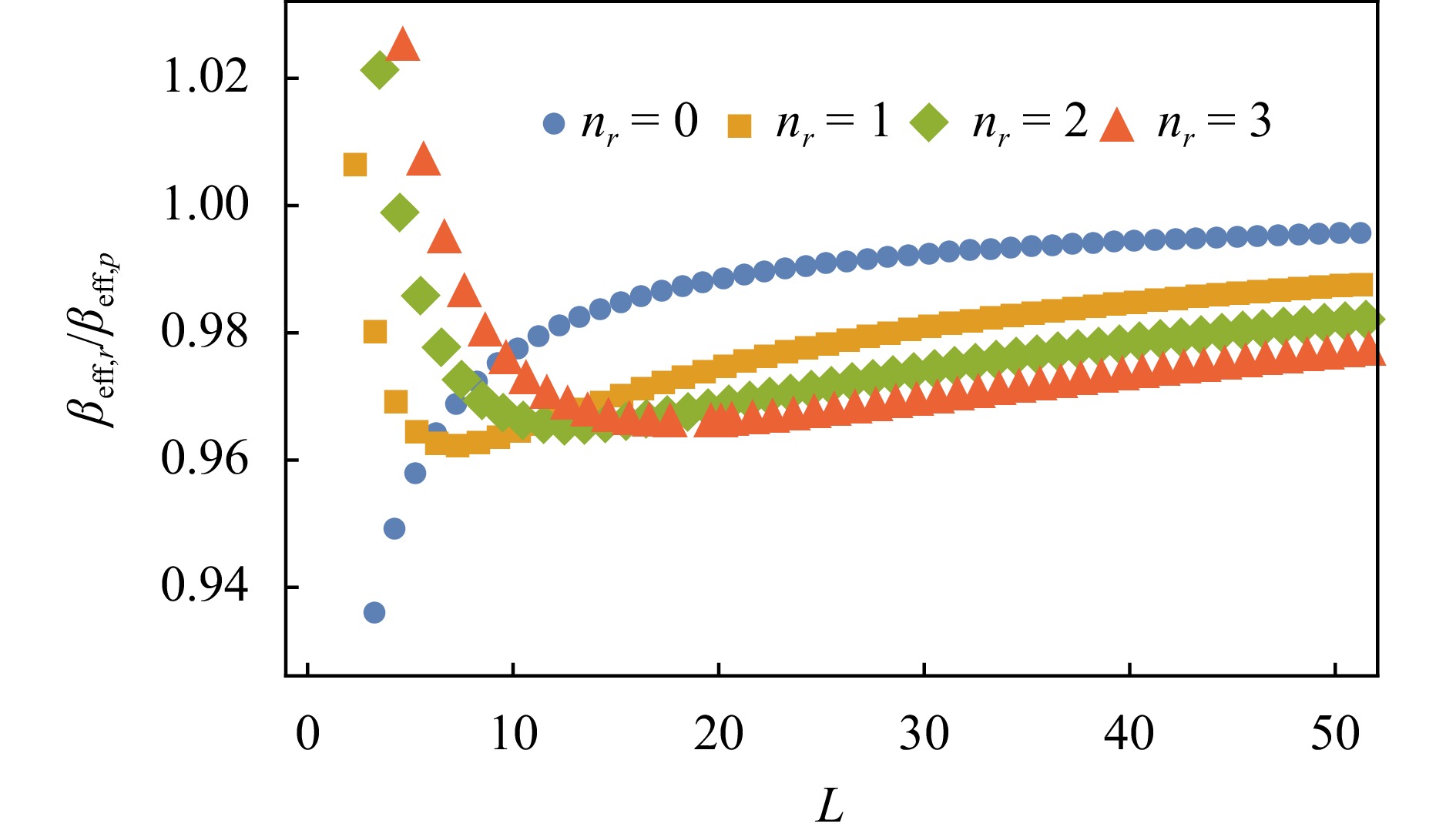
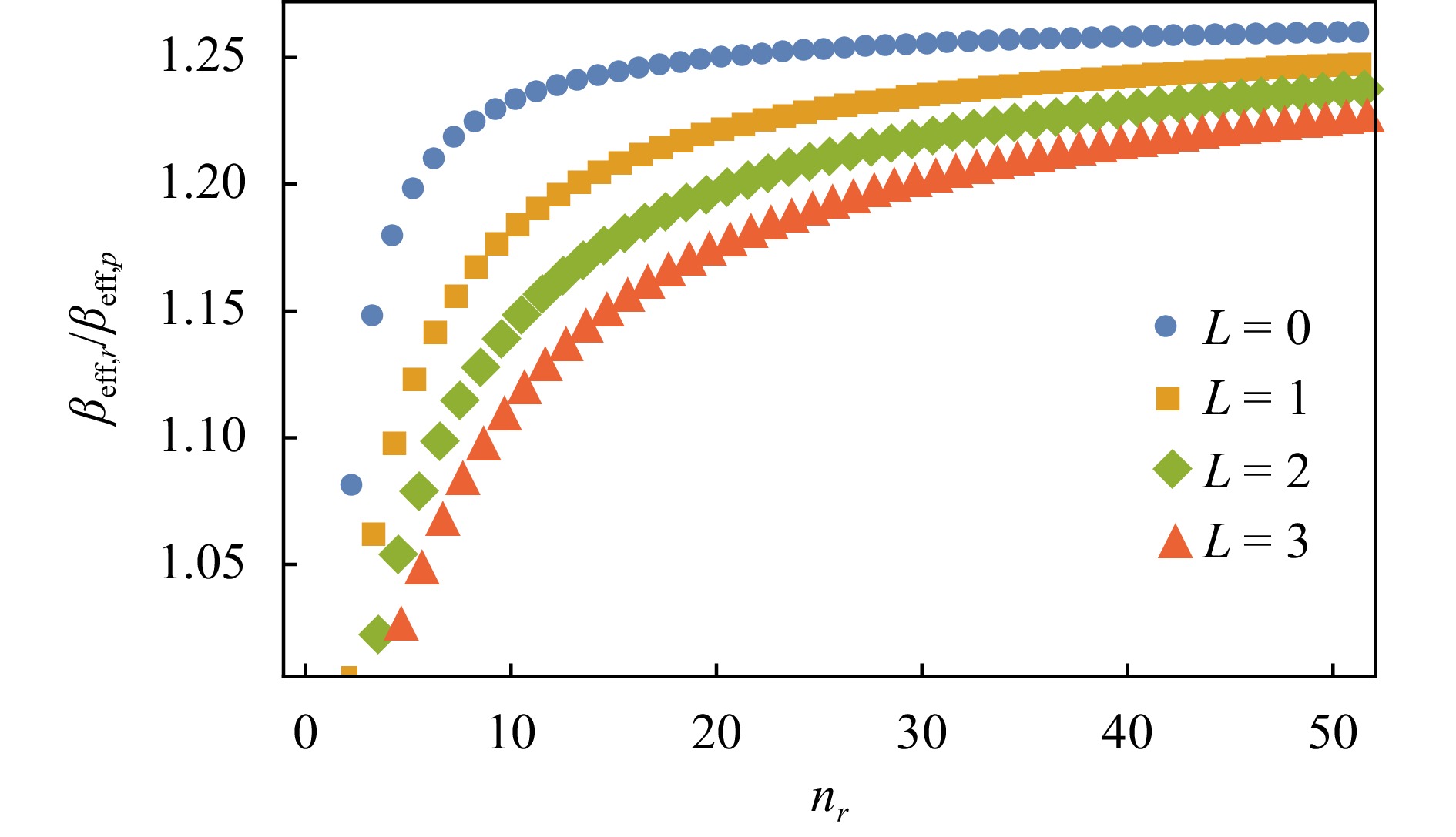
$ L $ is finite and$ n_r $ tends to infinity,${\beta_{{\rm eff}, \, {{{\boldsymbol{r}}}}}}/{\beta_{{\rm eff}, \, {{{\boldsymbol{p}}}}}}=2\sqrt{\frac{2}{5}}\approx 1.264\;9$ .2) When
$ n_r $ is finite and$ L $ tends to infinity,$ {\beta_{{\rm eff}, \, {{{\boldsymbol{r}}}}}}/{\beta_{{\rm eff}, \, {{{\boldsymbol{p}}}}}}=1 $ .We draw the curve of
$ \beta_{{\rm eff}, \, {{{\boldsymbol{r}}}}}/\beta_{{\rm eff}, \, {{{\boldsymbol{p}}}}} $ when$ L =(0, 3) $ ,$ n_r=(0, 50) $ and$ n_r =(0, 3) $ ,$ L=(0, 50) $ , respectively, as shown in Fig. 1 and Fig. 2. In Fig. 1 and Fig. 2, when we take the larger value of$ n_r(L) $ , the value of$ \beta_{{\rm eff}, \, {{{\boldsymbol{r}}}}}/\beta_{{\rm eff}, \, {{{\boldsymbol{p}}}}} $ is closer to 1.264 9. In addition, we bring these formulas into the Hamiltonian equation satisfied by the wave function of hydrogen atom to obtain$ \beta_{{\rm eff}, \, {{{\boldsymbol{r}}}}}, \; \beta_{{\rm eff}, \, {{{\boldsymbol{p}}}}} $ and$ \beta_{{\rm eff}, \, {{{\boldsymbol{r}}}}}/\beta_{{\rm eff}, \, {{{\boldsymbol{p}}}}} $ , the results are list in Table 1. It can be seen from Fig. 1, Fig. 2 and Table 1 that in most cases, when$ n_r < L $ ,$ \beta_{{\rm eff}, \, {{{\boldsymbol{r}}}}}/\beta_{{\rm eff}, \, {{{\boldsymbol{p}}}}} < 1 $ , and when$ n_r > L $ ,$ \beta_{{\rm eff}, \, {{{\boldsymbol{r}}}}}/\beta_{{\rm eff}, \, {{{\boldsymbol{p}}}}} > 1 $ . In Table 1, we use the result of the exact solution of the$ \beta_{\rm eff} $ value Eq. (32) under the hydrogen atom wave function to verify the result of the$ \beta_{\rm eff} $ value of the Eq. (26) when the harmonic oscillator basis is expanded. The data in the Table 1 show that the Eq. (26) is correct. (It should be noted that in the calculation process of the vector basis expansion in this paper, the size of the matrix taken is$ 16\times 16 $ . If the number of matrix vector basis is more, the data will be more accurate.)
Figure 1. (color online) The curve of
$ \beta_{{\rm eff}, \, {{{\boldsymbol{r}}}}}/\beta_{{\rm eff}, \, {{{\boldsymbol{p}}}}} $ when L = (0, 3), nr=(0, 50).Table 1.
$\beta_{{\rm eff}, \, {\boldsymbol{r}}}, \beta_{{\rm eff}, \, {\boldsymbol{p}}} \, {\rm and}$ energy spectrum value in the wave function of hydrogen atom.keV $n_r$ $L$ ${\rm state}(nl)$ Exact solution Numerical solution (SHO-expednded) $\beta_{{\rm eff}, \, {\boldsymbol{r}}}$ $\beta_{{\rm eff}, \, {\boldsymbol{p}}}$ $\beta_{{\rm eff}, \, {\boldsymbol{r}}}/ \beta_{{\rm eff}, \, {\boldsymbol{p}}}$ $E$ $\beta_{{\rm eff}, \, {\boldsymbol{r}}}$ $\beta_{{\rm eff}, \, {\boldsymbol{p}}}$ $\beta_{{\rm eff}, \, {\boldsymbol{r}}}/ \beta_{{\rm eff}, \, {\boldsymbol{p}}}$ $E$ 0 0 1S 2.637 5 3.045 5 0.866 0 −13.612 9 2.663 0 3.039 9 0.876 0 −13.563 9 0 1 2P 1.076 7 1.179 5 0.912 9 −3.403 2 1.079 0 1.179 0 0.915 1 −3.401 3 0 2 3D 0.621 7 0.664 6 0.935 4 −1.512 5 0.622 0 0.664 5 0.936 1 −1.512 3 0 3 4F 0.417 0 0.439 6 0.948 7 −0.850 8 0.417 2 0.439 6 0.949 0 −0.850 8 0 4 5G 0.304 5 0.318 1 0.957 4 −0.544 5 0.304 6 0.318 1 0.957 6 −0.544 5 1 0 2S 1.076 7 0.996 9 1.080 1 −3.403 2 1.090 3 0.988 6 1.103 0 −3.403 2 1 1 3P 0.589 8 0.586 1 1.006 2 −1.512 5 0.593 2 0.584 7 1.014 5 −1.512 5 1 2 4D 0.389 6 0.397 6 0.980 0 −0.850 8 0.390 8 0.397 3 0.983 6 −0.850 8 1 3 5F 0.283 5 0.292 6 0.969 0 −0.544 5 0.283 9 0.292 5 0.970 8 −0.544 5 2 0 3S 0.608 0 0.530 1 1.146 8 −1.512 5 0.608 9 0.515 8 1.180 6 −1.512 5 2 1 4P 0.388 2 0.365 7 1.061 4 −0.850 8 0.392 4 0.362 4 1.082 7 −0.850 8 2 2 5D 0.278 0 0.272 4 1.020 6 −0.544 5 0.280 6 0.271 5 1.033 4 −0.544 5 
Figure 2. (color online) The curve of
$ \beta_{{\rm eff}, \, {{{\boldsymbol{r}}}}}/\beta_{{\rm eff}, \, {{{\boldsymbol{p}}}}} $ when nr = (0, 3), L=(0, 50). -
In order to make a comparison with the numerical results of close[26], the potential and parameters used in the calculation are consistent with those in Ref. [26]:
$$ V(r)=\frac{4}{3}C_{q\bar{q}}-\frac{4}{3}\frac{\alpha_s}{r}+br+\frac{32\pi \alpha_s }{9 m_1 m_2}\tilde {\delta_{\sigma}}(r){\boldsymbol{S}}_1\boldsymbol\cdot {\boldsymbol{S}}_2, $$ (34) and
$ \tilde{\delta}_{\sigma}(r)=(\frac{\sigma}{\sqrt{\pi}})^3{\rm e}^{-\sigma^2r^2} $ . Where parameters used for the calculation are listed as follows[26]:$ C_{us}=-0.500 $ GeV,$ C_{uu}=-0.330 $ GeV, b= 0.162$ \; \rm GeV^2 $ ,$ \alpha $ = 0.594,$ \sigma $ = 0.897 GeV,$ m_u $ = 0.33 GeV,$ m_c $ = 1.6 GeV. The following calculations are listed as an example of a system consisting of$ u\bar{u} $ quark and$ u\bar{s} $ quark.The behavior of
$ \beta_{\rm eff} $ is discussed below. Our analytical results are compared with those in Ref. [26]. -
The QPC model was first proposed by Micu[27]. After decades of further development[28-34], the model has been widely used to calculate the strong two-body decay allowed by Okubo-Zweig-Iizuka(OZI) rule. In the QPC model, the transition matrix of the decay process
$ A\to B+C $ is defined by$$ \begin{array}{l} \langle BC|\mathcal{T}|A \rangle = \delta ^3({\boldsymbol{P}}_B+{\boldsymbol{P}}_C)\mathcal{M}^{{M}_{J_{A}}M_{J_{B}}M_{J_{C}}}, \end{array} $$ (35) where
$ A $ represents the initial state particle,$ B $ and$ C $ represent the final state particle formed after the decay of the initial state particle$ A $ .$ \mathcal{M}^{{M}_{J_{A}}M_{J_{B}}M_{J_{C}}} $ is the amplitude of$ A\to B+C $ .$ \mathcal{T} $ is the transition operator, which can describe the quark-antiquark pair generated from the vacuum. It can be expressed as$$ \begin{split} \mathcal{T} =& -3\gamma \sum\limits_{m}\langle 1m;1\; -m|00\rangle\int {\rm d} {\boldsymbol{p}}_3{\rm d}{\boldsymbol{p}}_4\delta ^3 ({\boldsymbol{p}}_3+{\boldsymbol{p}}_4) \times \\& \mathcal{Y}_{1m}\left(\frac{{\boldsymbol{p}}_3-{\boldsymbol{p}}_4}{2}\right)\chi _{1, -m}^{34}\phi _{0}^{34} \left(\omega_{0}^{34}\right)_{ij}b_{3i}^{\dagger}({\boldsymbol{p}}_3)d_{4j}^{\dagger}({\boldsymbol{p}}_4){, } \end{split} $$ (36) in the formula (36), the subscripts 3 and 4 represent quark and antiquark, respectively.
$ \chi $ ,$ \phi $ and$ \omega $ represent spin, taste and color wave functions of particle, respectively.$ \gamma $ is a dimensionless constant, which describes the generation rate of positive and negative quark pairs in vacuum, and it is generally determined by fitting experimental data.$ \mathcal{Y}_{\ell m}({\boldsymbol{p}})={|{\boldsymbol{p}}|^{\ell}}Y_{\ell m}({\boldsymbol{p}}) $ is the solid harmonic. According to the Jacobi-Wick formula, the helicity amplitude is converted into the partial wave amplitude, and the amplitude is expressed as$$ \begin{split} \mathcal{M}^{J L}({\boldsymbol{P}})=& \frac{\sqrt{4 \pi(2 L+1)}}{2 J_{A}+1} \sum\limits_{M_{J_{B}} M_{J_{C}}}\langle L 0 ; J M_{J_{A}} \mid J_{A} M_{J_{A}}\rangle\times \\& \langle J_{B} M_{J_{B}} ; J_{C} M_{J_{C}} \mid J_{A} M_{J_{A}}\rangle \mathcal{M}^{M_{J_{A}} M_{J_{B}} M_{J_{C}}}. \end{split} $$ (37) Therefore, the decay width of
$ A \rightarrow B C $ is read as$$ \begin{align} \varGamma=\frac{\pi}{4} \frac{|P|}{m_{A}^{2}} \sum_{J,\; L}\left|M^{J L}(\boldsymbol{P})\right|^{2}, \end{align} $$ (38) where
$ {\rm{m}}_{A} $ is the mass of the initial state A-meson.In addition, the meson wave function is defined as mock state,
$ i. e $ .$$ \begin{split} |A\left( {{n}^{2S+1}}{{L}_{J{{M}_{J}}}} \right)&\left( {{\boldsymbol{p}}_{A}} \right)=\sqrt{2E}\sum\limits_{{{M}_{S}},\, {{M}_{L}}}{}\langle L{{M}_{L}}S{{M}_{S}}|J{{M}_{J}}\rangle \times \\&\chi _{S{{M}_{S}}}^{A}{{\phi }^{A}}{{\omega }^{A}}\int{\text{d}}{{\boldsymbol{p}}_{1}}\text{d}{{\boldsymbol{p}}_{2}}{{\delta }^{3}}\left( {{\boldsymbol{p}}_{A}}-{{\boldsymbol{p}}_{1}}-{{\boldsymbol{p}}_{2}} \right)\times \\&\varPsi_{nL{{M}_{L}}}^{A}\left( {{\boldsymbol{p}}_{1}},\, {{\boldsymbol{p}}_{2}} \right)|{{q}_{1}}\left( {{\boldsymbol{p}}_{1}} \right){{\bar{q}}_{2}}\left( {{\boldsymbol{p}}_{2}} \right)\rangle , \end{split} $$ (39) where
$ M_L, \; L, \; J\; $ are magnetic quantum number, orbital angular momentum quantum number and total angular momentum quantum number respectively. It should be noted that here the spatial wave function$ \psi_{n L M_{L}}({\boldsymbol{p}}) $ of the meson is the SHO wave function in momentum space.The QPC model is calculated in momentum space, the
$ \beta_{\rm eff} $ in wave function here should also be more reasonable from momentum space. However the$ \beta_{\rm eff} $ of coordinate space is widely used in previous calculations[7-18, 20]. It is necessary to investigate the difference of results of the QPC model with$ \beta_{{\rm eff}, \, {\boldsymbol{r}}} $ and$ \beta_{{\rm eff}, \, {\boldsymbol{p}}} $ . -
Case 1:
$ \beta $ =0.4 GeVWhen
$ \beta $ in the exact wave function takes the common value 0.4 GeV as the input, the corresponding$ \beta_{\rm eff} $ values are obtained according to Eq. (26) as shown in Table 2 and Table 3.Table 2. The
$ \beta_{\rm eff} $ value of$ u\bar{u} $ quark system when$ \beta $ takes the common value of 0.4 GeV.GeV State $\beta_{{\rm eff}, \, {\boldsymbol{r}}}$ $\beta_{{\rm eff}, \, {\boldsymbol{r}}}$[26] $\beta_{{\rm eff}, \, {\boldsymbol{p}}}$ State $\beta_{{\rm eff}, \, {\boldsymbol{r}}}$ $\beta_{{\rm eff}, \, {\boldsymbol{r}}}$[26] $\beta_{{\rm eff}, \, {\boldsymbol{p}}}$ $0^1S_0$ 0.476 0 0.47 0.540 5 $0^3S_1$ 0.283 7 0.28 0.285 0 $1^1S_0$ 0.280 1 0.28 0.271 0 $1^3S_1$ 0.241 2 0.24 0.239 1 $2^1S_0$ 0.241 1 0.24 0.234 2 $2^3S_1$ 0.222 9 0.23 0.221 2 $3^1S_0$ 0.226 9 0.222 8 $3^3S_1$ 0.220 6 0.222 2 $0^1P_1$ 0.271 5 0.27 0.276 1 $0^3P_J$ 0.263 0 0.26 0.264 4 $1^1P_1$ 0.238 7 0.241 4 $1^3P_J$ 0.232 6 0.232 0 $2^1P_1$ 0.223 9 0.225 9 $2^3P_J$ 0.219 5 0.219 0 $3^1P_1$ 0.227 8 0.232 6 $3^3P_J$ 0.225 8 0.229 6 $0^1D_2$ 0.246 9 0.25 0.247 9 $0^3D_J$ 0.246 4 0.25 0.247 4 $1^1D_2$ 0.225 4 0.225 7 $1^3D_J$ 0.224 9 0.225 0 $2^1D_2$ 0.218 8 0.220 2 $2^3D_J$ 0.218 3 0.219 5 $3^1D_2$ 0.233 9 0.239 0 $3^3D_J$ 0.233 6 0.238 6 Table 3. The
$\beta_{\rm eff}$ value of$u\bar{s}$ quark system when$\beta$ takes the common value of 0.4 GeV.GeV State $\beta_{{\rm eff}, \, {\boldsymbol{r}}}$ $\beta_{{\rm eff}, \, {\boldsymbol{r}}}$[26] $\beta_{{\rm eff}, \, {\boldsymbol{p}}}$ State $\beta_{{\rm eff}, \, {\boldsymbol{r}}}$ $\beta_{{\rm eff}, \, {\boldsymbol{r}}}$[26] $\beta_{{\rm eff}, \, {\boldsymbol{p}}}$ $0^1S_0$ 0.453 5 0.46 0.502 4 $0^3S_1$ 0.3155 0.32 0.3179 $1^1S_0$ 0.294 2 0.29 0.289 6 $1^3S_1$ 0.263 8 0.26 0.261 6 $2^1S_0$ 0.256 3 0.25 0.251 3 $2^3S_1$ 0.241 7 0.24 0.239 6 $3^1S_0$ 0.238 7 0.234 7 $3^3S_1$ 0.231 4 0.230 4 $0^1P_1$ 0.293 9 0.29 0.298 4 $0^3P_J$ 0.285 9 0.29 0.287 6 $1^1P_1$ 0.257 4 0.259 5 $1^3P_J$ 0.251 8 0.251 2 $2^1P_1$ 0.239 2 0.240 1 $2^3P_J$ 0.235 0 0.233 9 $3^1P_1$ 0.233 5 0.235 4 $3^3P_J$ 0.231 0 0.231 8 $0^1D_2$ 0.267 3 0.27 0.268 5 $0^3D_J$ 0.266 8 0.27 0.267 9 $1^1D_2$ 0.243 2 0.243 5 $1^3D_J$ 0.242 6 0.242 7 $2^1D_2$ 0.231 0 0.231 2 $2^3D_J$ 0.230 4 0.230 4 $3^1D_2$ 0.234 6 0.237 6 $3^3D_J$ 0.234 2 0.237 0 From Table 2 and Table 3, it can be seen that
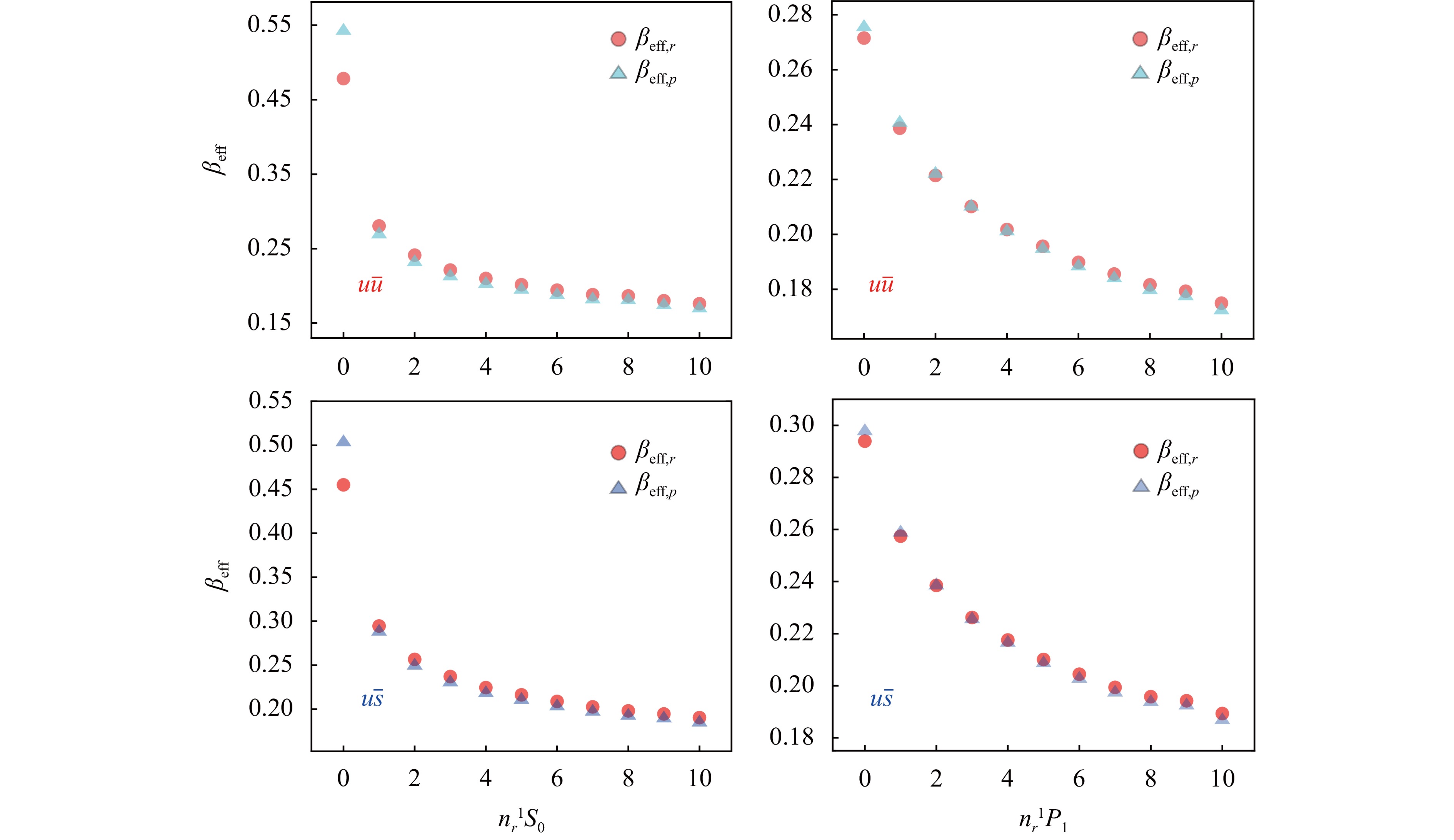
$ \beta_{{\rm eff}, \, {\boldsymbol{r}}} $ and$ \beta_{{\rm eff}, \, {\boldsymbol{p}}} $ of mesons in the ground state are significantly different. For example, for the ground state ($ 0^1S_0 $ ) of the$ u\bar{u} $ meson system,$ \beta_{{\rm eff}, \, {\boldsymbol{r}}}= 0.476\; 0 $ GeV,$ \beta_{{\rm eff}, \, {\boldsymbol{p}}} = 0.540\; 5 $ GeV; for the ground state ($ 0^1S_0 $ ) of the$ u\bar{s} $ meson system,$ \beta_{{\rm eff}, \, {\boldsymbol{r}}} = 0.453\; 5 $ GeV,$ \beta_{{\rm eff}, \, {\boldsymbol{p}}} = 0.502\; 4 $ GeV. From the above two sets of data, we can see that when the meson is in the ground state, the$ \beta_{\rm eff} $ obtained in coordinate space and momentum space are significantly different, while in the highly excited states,$ \beta_{{\rm eff}, \, {\boldsymbol{r}}} $ and$ \beta_{{\rm eff}, \, {\boldsymbol{p}}} $ are relatively close.Case 2: variable
$ \beta $ Taking
$ \beta $ as a function of energy, the$ \beta $ at the lowest ground state energy is obtained by the variational method. Then the$ \beta_{\rm eff} $ value in corresponding coordinate space and momentum space will produced by solving Eq. (26). As shown in Table 4 and Table 5, the results obtained with the$ \beta $ selected in this way are consistent with those obtained with$ \beta $ = 0.4 GeV. This further demonstrates the appropriateness of using$ \beta=0.4 $ GeV as the input for the numerical calculation of$ \beta_{\rm eff} $ in all previous references. Similarly, we can still see from the Table 4 and Table 5 that$ \beta_{{\rm eff}, \, {\boldsymbol{r}}} $ differs greatly from$ \beta_{{\rm eff}, \, {\boldsymbol{p}}} $ in the ground state. The behavior of$ \beta_{{\rm eff}, \, {\boldsymbol{r}}} $ and$ \beta_{{\rm eff}, \, {\boldsymbol{p}}} $ are similar in the highly excited state.Table 4. The
$ \beta_{\rm eff} $ value of the$ u\bar{u} $ quark system corresponding to case 2.GeV ${\rm State}$ $\beta$ $\beta_{{\rm eff}, \, {\boldsymbol{r}}}$ $\beta_{{\rm eff}, \, {\boldsymbol{r}}} $[26] $\beta_{{\rm eff}, \, {\boldsymbol{p}}}$ $\rm State$ $\beta$ $\beta_{{\rm eff}, \, {\boldsymbol{r}}}$ $\beta_{{\rm eff}, \, {\boldsymbol{r}}} $[26] $\beta_{{\rm eff}, \, {\boldsymbol{p}}}$ $0^1S_0$ $0.702\; 0$ $0.478 \;3$ $0.47$ $0.545\; 2$ $0^3S_1$ $0.468\; 1$ $0.283\; 7$ $0.28$ $0.285\; 0$ $1^1S_0$ $0.487 \;6$ $0.280 \;5$ $0.28$ $0.271\; 8$ $1^3S_1$ $0.312\; 1$ $0.241\; 2$ $0.24$ $0.239 \;1$ $2^1S_0$ $0.409 \;6$ $0.241\; 3$ $0.24$ $0.234 \;5$ $2^3S_1$ $0.312 \;1$ $0.222\; 1$ $0.23$ $0.220 \;1$ $3^1S_0$ $0.312 \;1$ $0.221 \;2$ $0.215 \;4$ $3^3S_1$ $0.292 6$ $0.210\; 2$ $0.208 \;4$ $0^1P_1$ $0.468 \;1$ $0.271\; 5$ $0.27$ $0.276\; 2$ $0^3P_J$ $0.390 \;1$ $0.263\; 0$ $0.26$ $0.264\; 4$ $1^1P_1$ $0.390\; 1$ $0.238 \;7$ $0.241\; 4$ $1^3P_J$ $0.312\; 1$ $0.232\; 5$ $0.231\; 9$ $2^1P_1$ $0.312\;1$ $0.221\;4$ $0.222\;8$ $2^3P_J$ $0.312\; 1$ $0.216\; 7$ $0.215\; 6$ $3^1P_1$ $0.312\; 1$ $0.210\; 2$ $0.210\; 8$ $3^3P_J$ $0.273\; 1$ $0.2063$ $0.205\; 0$ $0^1D_2$ $0.312\; 1$ $0.246\; 8$ $0.25$ $0.247 9$ $0^3D_J$ $0.312 \;1$ $0.246\; 4$ $0.25$ $0.247\; 4$ $1^1D_2$ $0.312\; 1$ $0.225\; 0$ $0.225 \;2$ $1^3D_J$ $0.292\; 6$ $0.224\; 4$ $0.224\; 5$ $2^1D_2$ $0.312\; 1$ $0.212\; 1$ $0.212\; 0$ $2^3D_J$ $0.273 \;1$ $0.211 \;6$ $0.211 \;1$ $3^1D_2$ $0.273\;1$ $0.203\;1$ $0.202\;7$ $3^3D_J$ $0.253\; 7$ $0.202\; 6$ $0.201\; 9$ Table 5. The
$ \beta_{\rm eff} $ value of the$ u\bar{s} $ quark system corresponding to case 2.GeV ${\rm State}$ $\beta$ $\beta_{{\rm eff}, \, {\boldsymbol{r}}}$ $\beta_{{\rm eff}, \, {\boldsymbol{r}}} $[26] $\beta_{{\rm eff}, \, {\boldsymbol{p}}}$ $\rm{ State}$ $\beta$ $\beta_{{\rm eff}, \, {\boldsymbol{r}}}$ $\beta_{{\rm eff}, \, {\boldsymbol{r}}} $[26] $\beta_{{\rm eff}, \, {\boldsymbol{p}}}$ $0^1S_0$ $0.702\; 0$ $0.455 \; 1$ $0.46$ $0.505 \; 7$ $0^3S_1$ $0.565 \; 5$ $0.315 \; 5$ $0.32$ $0.318 \; 0$ $1^1S_0$ $0.507 \; 1$ $0.294 \; 6$ $0.29$ $0.290 \; 3$ $1^3S_1$ $0.448 \; 6$ $0.263 \; 8$ $0.26$ $0.261 \; 6$ $2^1S_0$ $0.429 \; 1$ $0.256 \; 6$ $0.25$ $0.251 8$ $2^3S_1$ $0.312 \; 1$ $0.241 \; 6$ $0.24$ $0.239 \; 5$ $3^1S_0$ $0.370 \; 6$ $0.237 \; 1$ $0.232 \; 7$ $3^3S_1$ $0.312 \; 1$ $0.228 \; 0$ $0.226 \; 1$ $0^1P_1$ $0.468 \; 1$ $0.293 \; 9$ $0.29$ $0.298 \; 5$ $0^3P_J$ $0.390 \; 1$ $0.285 \; 9$ $0.29$ $0.287 \; 6$ $1^1P_1$ $0.429 \; 1$ $0.257 \; 4$ $0.259 \; 6$ $1^3P_J$ $0.312 \; 1$ $0.251 \; 8$ $0.251 \; 2$ $2^1P_1$ $0.312 \; 1$ $0.238 \; 5$ $0.239 \; 3$ $2^3P_J$ $0.312 \; 1$ $0.234 \; 4$ $0.233 \; 2$ $3^1P_1$ $0.312 \; 1$ $0.226 \; 2$ $0.226 \; 3$ $3^3P_J$ $0.273 \; 1$ $0.222 \; 9$ $0.221 6$ $0^1D_2$ $0.409 \; 6$ $0.267 \; 3$ $0.27$ $0.268 \; 5$ $0^3D_J$ $0.370 \; 6$ $0.266 \; 8$ $0.27$ $0.267 \; 9$ $1^1D_2$ $0.312 \; 1$ $0.243 \; 1$ $0.243 \; 4$ $1^3D_J$ $0.292 \; 6$ $0.242 \; 6$ $0.242 \; 6$ $2^1D_2$ $0.312 \; 1$ $0.229 \; 0$ $0.228 \; 8$ $2^3D_J$ $0.292 \; 6$ $0.228 \; 5$ $0.228 0$ $3^1D_2$ $0.312 \; 1$ $0.219 \; 3$ $0.218 \; 8$ $3^3D_J$ $0.273 \; 1$ $0.218 \; 7$ $0.217 \; 9$ In addition, we draw the curves of
$ \beta_{{\rm eff}, \, {\boldsymbol{r}}} $ and$ \beta_{{\rm eff}, \, {\boldsymbol{p}}} $ for different radial quantum numbers ($ n_r $ ) of the same orbital quantum number (L) in Fig. 3. From the figure, we can see that the values of$ \beta_{{\rm eff}, \, {\boldsymbol{r}}} $ and$ \beta_{{\rm eff}, \, {\boldsymbol{p}}} $ coincide in the highly excited state. It is permissible to replace the behavior of$ \beta_{{\rm eff}, \, {\boldsymbol{p}}} $ with$ \beta_{{\rm eff}, \, {\boldsymbol{r}}} $ in the QPC model. However, the behavior of both in the ground state tells us that when using QPC to calculate the decay amplitude, it is necessary to be careful to select$ \beta_{\rm eff} $ as the calculation parameter if the effective SHO wave function is for the ground state.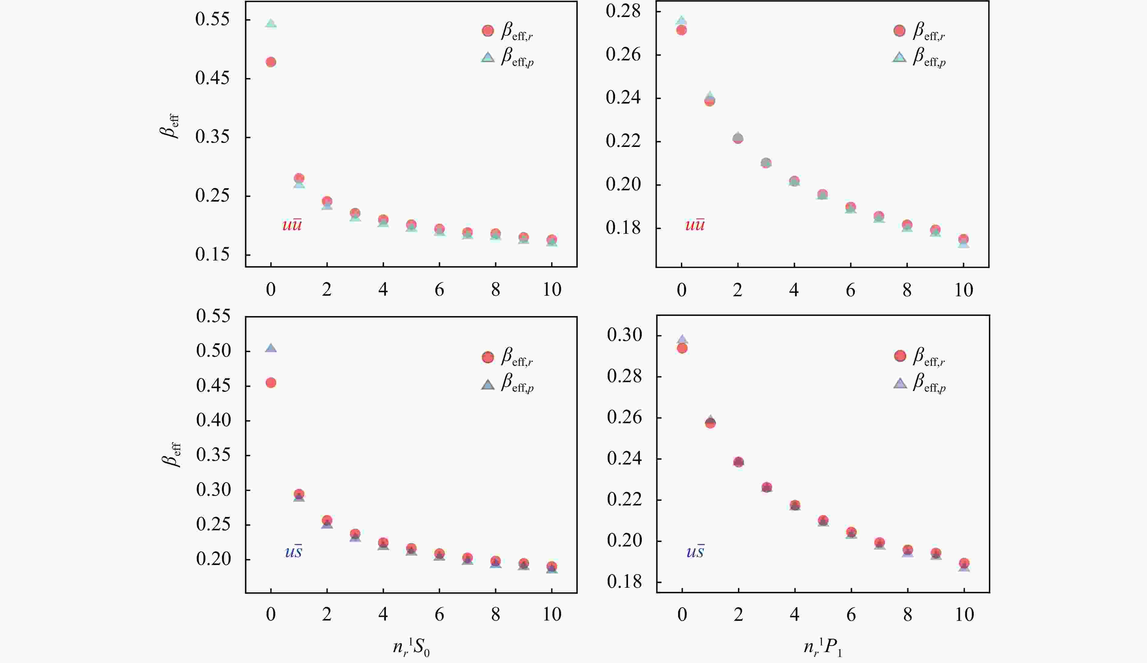
Figure 3. (color online) Graphs of
$ \beta_{\rm eff} $ value of the$ u\bar{u} $ and$ u\bar{s} $ quark systems when$ \beta $ is taken at lowest energy, where the abscissa represents the radial quantum number$ n_r $ , and the ordinate is the magnitude of$ \beta_{{\rm eff}, \, {\boldsymbol{r}}} $ and$ \beta_{{\rm eff}, \, {\boldsymbol{p}}} $ , in units of GeV.We use
$ \beta_{{\rm eff}, \, {\boldsymbol{r}}} $ and$ \beta_{{\rm eff}, \, {\boldsymbol{p}}} $ as the parameter in the effective SHO wave function of the QPC model to calculate several decay channels, which are in the ground states. The decay channels and quark mass obtained are from Ref. [11]. The results are shown in Table 6.Table 6. Comparison of the decay widths calculated by QPC model with
$ \beta_{\rm eff} $ from coordinate space and momentum space, and the results are obtained in the QPC model when$ m_u=m_d=0.33 $ GeV and$ m_s=0.55 $ GeV, the unit of width is MeV.${\rm Decay\; channel}$ ${\rm Measured}$[35] $\beta_ {{\rm eff}, \, {\boldsymbol{r}}}$ $\beta_ {{\rm eff}, \, {\boldsymbol{p}}}$ ${\rm Decay\; channel}$ ${\rm Measured}$[35] $\beta_ {{\rm eff}, \, {\boldsymbol{r}}}$ $\beta_ {{\rm eff}, \, {\boldsymbol{p}}}$ $b_1(1235)\to \omega \pi$ $142 \pm 8$ $118.106$ $125.297$ $K^*(892)\to K\pi$ $48.7 \pm 0.8$ $ 28.029 $ $27.245$ $\phi\to K^+K^-$ $2.08 \pm 0.02$ $1.908$ $2.010$ $K^*(1410)\to K\pi$ $15.3 \pm 1.4$ $11.307$ $27.623$ $a_2(1320)\to \eta \pi$ $15.5 \pm 0.7$ $21.280$ $13.525$ $K^*_0(1430)\to K\pi$ $251 \pm 74$ $165.174$ $258.416$ $a_2(1320)\to K\bar{K}$ $5.2 \pm 0.2$ $2.277$ $1.638$ $K^*_2(1430)\to K\pi$ $54.4 \pm 2.5$ $64.803$ $49.188$ $\pi_2(1670)\to f_2(1270)\pi$ $145.8 \pm 5.1$ $135.914$ $151.546$ $K^*_2(1430)\to K^*(892)\pi$ $26.9 \pm 1.2$ $31.526$ $29.538$ $\rho_3(1690)\to \pi\pi$ $38 \pm 2.4$ $32.801$ $15.528$ $K^*_2(1430)\to K\rho$ $9.5 \pm 0.4$ $14.022$ $14.248$ $\rho_3(1690)\to \omega \pi$ $25.8 \pm 1.6$ $65.359$ $57.558$ $K^*_2(1430)\to K\omega$ $3.16 \pm 0.15$ $4.292$ $4.361$ $\rho_3(1690)\to K\bar{K}$ $2.5 \pm 0.2$ $1.330$ $0.728$ $\chi^2=1913$ $\chi^2=1914$ $\gamma=8.663$ $\gamma=9.871$ It can be seen from Table 6 that
$ \beta_ {{\rm eff}, \, {\boldsymbol{r}}} $ obtained from coordinate space and$ \beta_ {{\rm eff}, \, {\boldsymbol{p}}} $ from momentum space have great influence on the calculation results of decay width when a SHO wave function is taken as effective wave function in QPC model. Compared with Ref. [11], the decay width calculated from coordinate space is close to the data of Ref. [11].What is more noteworthy in Table 6 is that, we found that when
$ \beta_{\rm eff} $ is taken from different spaces, it has a great influence on the vacuum generation rate$ \gamma $ and decay width. Firstly, the$ \gamma $ obtained by fitting in$ \beta_ {{\rm eff}, \, {\boldsymbol{r}}} $ is 12% less than it by fitting$ \beta_ {{\rm eff}, \, {\boldsymbol{p}}} $ . The$ \beta_ {{\rm eff}, \, {\boldsymbol{r}}} $ and$ \beta_ {{\rm eff}, \, {\boldsymbol{p}}} $ of the highly excited states are roughly equal, but the$ \gamma $ value obtained from different spaces are highly correlated with the decay width, which also makes the difference between the two result of width which obtained from coordinate space and momentum space reach about 20% in some decays containing the highly excited states. Secondly, the average relative error between the decay width obtained from the$ \beta_ {{\rm eff}, \, {\boldsymbol{r}}} $ and the$ \beta_ {{\rm eff}, \, {\boldsymbol{p}}} $ with the experimental value is calculated. The formula is as follows$$ \overline{RE}=\frac{1}{15}\sum\limits_{i=1}^{15} \frac{|\varGamma_i(\beta_ {{\rm eff}, \, {\boldsymbol{r}}})-\varGamma_i(\beta_ {{\rm eff}, \, {\boldsymbol{p}}})|}{\varGamma_i({\rm Exp})}, $$ (40) and the
$ \overline{RE}=0.245\; 9 $ . This means that the difference is about 25% using$ \beta_ {{\rm eff}, \, {\boldsymbol{r}}} $ and$ \beta_ {{\rm eff}, \, {\boldsymbol{p}}} $ to calculate the decay width, respectively. This will have important implications for the use of QPC model.case 3:
$ \beta=\sqrt{\beta_{{\rm eff}, \, {\boldsymbol{r}}}\beta_{{\rm eff}, \, {\boldsymbol{p}}}} $ We discuss Eqs. (25) and (26) as follows. Since
$ \beta $ is theoretically arbitrary,$ \beta^2_{{\rm eff}, \, {\boldsymbol{r}}} $ and$ \beta_{{\rm eff}, \, {\boldsymbol{p}}}^2 $ are independent of$ \beta $ . We know from (26) that$ k_1-k_2 $ is equal to$ \beta^2 $ multiply some constant, and$ k_1+k_2 $ is equal to$ 1/\beta^2 $ multiply some constant. The relation between$ \beta_{{\rm eff}, \, {\boldsymbol{r}}} $ and$ \beta_{{\rm eff}, \, {\boldsymbol{p}}} $ will be obtained:$$ \beta^2_{{\rm eff}, \, {\boldsymbol{r}}}-\beta_{{\rm eff}, \, {\boldsymbol{p}}}^2=\dfrac{\beta^2 \Bigg[\left( { 2n_r+L+\dfrac{3}{2} } \right)^2-\left( { k_1^2-k_2^2 } \right)\Bigg]} {\left( { 2n_r+L+\dfrac{3}{2} } \right)(k_1-k_2)}, $$ (41) or
$$ \frac{\beta^2_{{\rm eff}, \, {\boldsymbol{r}}}}{\beta_{{\rm eff}, \, {\boldsymbol{p}}}^2}=\dfrac{\left( { 2n_r+L+\dfrac{3}{2} } \right)^2}{k_1^2-k_2^2}. $$ (42) The calculation is as follows from Eq. (26) :
$$\left\{ \begin{array}{l} \beta^{-2}_{{\rm eff}, \, {\boldsymbol{r}}}\left( { 2n_r+L+\dfrac{3}{2} } \right)=\beta^{-2}{(k_1-k_2)}, \\ \beta_{{\rm eff}, \, {\boldsymbol{p}}}^2\left( { 2n_r+L+\dfrac{3}{2} } \right)=\beta^2(k_1+k_2). \end{array} \right. $$ (43) If let
$ \beta^2=\beta_{{\rm eff}, \, {\boldsymbol{p}}}\beta_{{\rm eff}, \, {\boldsymbol{r}}} $ , the formula (43) can be written as$$\left\{ \begin{array}{l} \left( { 2n_r+L+\dfrac{3}{2} } \right)\dfrac{\beta_{{\rm eff}, \, {\boldsymbol{p}}}}{\beta_{{\rm eff}, \, {\boldsymbol{r}}}}=k_1-k_2, \\ \left( { 2n_r+L+\dfrac{3}{2} } \right)\dfrac{\beta_{{\rm eff}, \, {\boldsymbol{p}}}}{\beta_{{\rm eff}, \, {\boldsymbol{r}}}}=k_1+k_2. \end{array} \right. $$ (44) We find that the left side of Eq. (44) is equal, the right side is same only when
$ k_2= 0. $ i. e.$$ \left\{ \begin{array}{l} \beta=\sqrt{\beta_{{\rm eff}, \, {\boldsymbol{p}}}\beta_{{\rm eff}, \, {\boldsymbol{r}}}}.\\ k_2=2 \displaystyle \sum\limits_{n=0}^{N-2}c_{n}^*c_{n+1}\sqrt{(n+1)\Big(n+L+\frac{3}{2}\Big)}= 0\\ \dfrac{\beta_{{\rm eff}, \, {\boldsymbol{p}}}}{\beta_{{\rm eff}, \, {\boldsymbol{r}}}}=\dfrac{k_1}{2n_r+L+\dfrac{3}{2}}=\dfrac{ \displaystyle \sum\limits_{n=0}^{N-1}c_{n}^* c_{n}\Big(2n+L+\frac{3}{2}\Big)}{2n_r+L+\dfrac{3}{2}}. \end{array} \right. $$ (45) From Eq. (45), we also know that the average value of
$ n $ in the highly excited states ($ \beta_{{\rm eff}, \, {\boldsymbol{p}}}/\beta_{{\rm eff}, \, {\boldsymbol{r}}}\approx 1 $ ) is approximately equal to the radial quantum number$ n_r $ .In the specific calculation, we can do a cycle, so that
$ \beta $ approaches the square root of$ \sqrt{\beta_{{\rm eff}, \, {\boldsymbol{p}}}\beta_{{\rm eff}, \, {\boldsymbol{r}}}} $ . We test the relation (45) numerically. The cycles of$ k_2<10^{-3} $ ,$ \beta, \beta_{{\rm eff}, \; {\boldsymbol{r}}}, \; \beta_{{\rm eff}, \; {\boldsymbol{p}}}, \; \sqrt{\beta_{{\rm eff}, \;{\boldsymbol{p}}}\beta_{{\rm eff}, \; {\boldsymbol{r}}}}, \; k_2 $ and$ k_1 $ are listed in Table 7 and Table 8. It can be seen from Table 7 and Table 8 that when$ \beta=\sqrt{\beta_{{\rm eff}, \, {\boldsymbol{p}}}\beta_{{\rm eff}, \, {\boldsymbol{r}}}} $ , the sizes of$ \beta_{{\rm eff}, \, {\boldsymbol{r}}} $ and$ \beta_{{\rm eff}, \, {\boldsymbol{p}}} $ in the ground states are quite different, the sizes of them in the excited states are similar, which is consistent with the behavior of the previous two cases. The data in Table 7 and Table 8 also verifies the identity of$ k_2 = 0 $ , and$ k_1/2n_r+L+\frac{3}{2} \approx 1 $ , further verifies that the average value of$ n $ is approximately equal to the radial quantum number$ n_r $ at highly excited states.Table 7. Verification of the
$ k_2 $ value in the$ u\bar{u} $ quark system ($ S=0 $ ) and the$ \beta_{\rm eff} $ value when$ k_2<10^{-3} $ .${\rm State}$ $\beta$ $\beta_{{\rm eff}, \, {\boldsymbol{r}}}$ $\beta_{{\rm eff}, \, {\boldsymbol{p}}}$ $\sqrt{\beta_{{\rm eff}, \, {\boldsymbol{r}}}\beta_{{\rm eff}, \, {\boldsymbol{p}}}}$ $k_2$ $\dfrac{k_1}{2n_r+L+\dfrac{3}{2}}$ ${\rm Cycle\; index}$ $0^1S_0$ $0.509 \; 9$ $0.477 \; 6$ $0.544 \; 3$ $0.509 \; 9$ $1.421\times 10^{-4}$ $1.139 \; 5$ $2$ $1^1S_0$ $0.272 \; 1$ $0.277 \; 7$ $0.266 \; 6$ $0.272 \; 1$ $4.554\times 10^{-4}$ $0.960 \; 0$ $2$ $2^1S_0$ $0.233 \; 9$ $0.238 \; 4$ $0.229 \; 4$ $0.233 \; 9$ $1.267\times 10^{-4}$ $0.962 \; 1$ $2$ $3^1S_0$ $0.215 \; 8$ $0.219 \; 6$ $0.212 \; 1$ $0.215 \; 8$ $1.869\times 10^{-4}$ $0.966 \; 2$ $2$ $4^1S_0$ $0.204 \; 4$ $0.207 \; 7$ $0.201 \; 3$ $0.204 \; 4$ $1.921\times 10^{-6}$ $0.969 \; 3$ $2$ $5^1S_0$ $0.196 \; 1$ $0.199 \; 0$ $0.193 \; 3$ $0.196 \; 1$ $4.544\times 10^{-5}$ $0.971 \; 2$ $3$ $6^1S_0$ $0.189 \; 5$ $0.192 \; 2$ $0.186 \; 8$ $0.189 \; 5$ $1.117\times 10^{-5}$ $0.971 \; 8$ $3$ $0^1P_1$ $0.273 \; 3$ $0.271 \; 2$ $0.275 \; 4$ $0.273 \; 3$ $2.858\times 10^{-4}$ $1.015 \; 7$ $2$ $1^1P_1$ $0.237 \; 5$ $0.238 \; 2$ $0.240 \; 1$ $0.239 \; 1$ $8.002\times 10^{-4}$ $1.008 \; 0$ $2$ $2^1P_1$ $0.221 \; 3$ $0.221 \; 0$ $0.221 \; 6$ $0.221 \; 3$ $4.763\times 10^{-5}$ $1.002 \; 8$ $3$ $3^1P_1$ $0.209 \; 5$ $0.209 \; 6$ $0.209 \; 4$ $0.209 \; 5$ $7.539\times 10^{-5}$ $0.999 \; 1$ $3$ $4^1P_1$ $0.200 \; 8$ $0.201 \; 2$ $0.200 \; 5$ $0.200 \; 8$ $4.728\times 10^{-5}$ $0.996 \; 3$ $3$ $5^1P_1$ $0.194 \; 0$ $0.194 \; 6$ $0.193 \; 4$ $0.194 \; 0$ $2.040\times 10^{-4}$ $0.993 \; 9$ $3$ $6^1P_1$ $0.188 \; 2$ $0.189 \; 1$ $0.187 \; 4$ $0.188 \; 2$ $9.007\times 10^{-4}$ $0.991 \; 3$ $3$ $0^1D_2$ $0.247 \; 4$ $0.246 \; 8$ $0.247 \; 9$ $0.247 \; 4$ $2.066\times 10^{-5}$ $1.004 \; 2$ $2$ $1^1D_2$ $0.225 \; 1$ $0.225 \; 0$ $0.225 \; 2$ $0.225 \; 1$ $1.733\times 10^{-6}$ $1.001 \; 0$ $2$ $2^1D_2$ $0.212 \; 0$ $0.212 \; 1$ $0.211 \; 8$ $0.212 \; 0$ $4.953\times 10^{-5}$ $0.998 \; 8$ $2$ $3^1D_2$ $0.202 \; 8$ $0.203 \; 1$ $0.202 \; 6$ $0.202 \; 8$ $7.375\times 10^{-4}$ $0.997 \; 4$ $2$ $4^1D_2$ $0.195 \; 9$ $0.196 \; 2$ $0.195 \; 5$ $0.195 \; 9$ $1.225\times 10^{-5}$ $0.996 \; 4$ $3$ $5^1D_2$ $0.190 \; 3$ $0.190 \; 7$ $0.189 \; 8$ $0.190 \; 3$ $5.905\times 10^{-5}$ $0.995 \; 4$ $3$ $6^1D_2$ $0.185 \; 5$ $0.186 \; 0$ $0.184 \; 9$ $0.185 \; 5$ $1.663\times 10^{-4}$ $0.994 \; 3$ $3$ $0^1F_3$ $0.235 \; 3$ $0.235 \; 0$ $0.235 \; 6$ $0.235 \; 3$ $1.118\times10^{-6}$ $1.002 \; 8$ $2$ $1^1F_3$ $0.218 \; 0$ $0.217 \; 9$ $0.218 \; 1$ $0.218 \; 0$ $2.402\times 10^{-5}$ $1.001 \; 0$ $2$ $2^1F_3$ $0.206 \; 9$ $0.207 \; 0$ $0.206 \; 9$ $0.206 \; 9$ $8.741\times 10^{-5}$ $0.999 \; 2$ $2$ $3^1F_3$ $0.199 \; 0$ $0.199 \; 2$ $0.198 \; 7$ $0.199 \; 0$ $7.502\times 10^{-5}$ $0.997 \; 9$ $2$ $4^1F_3$ $0.192 \; 7$ $0.193 \; 0$ $0.192 \; 4$ $0.192 \;7$ $4.014\times 10^{-6}$ $0.996 \; 9$ $2$ $5^1F_3$ $0.187 \; 6$ $0.188 \; 0$ $0.187 \; 3$ $0.187 \;6$ $1.403\times 10^{-4}$ $0.996 \; 1$ $2$ $6^1F_3$ $0.183 \; 3$ $0.183 \; 7$ $0.182 \; 8$ $0.183 \;3$ $2.075\times 10^{-4}$ $0.995 \; 1$ $3$ $0^1G_4$ $0.226 \; 7$ $0.226 \; 5$ $0.227 \; 0$ $0.226 \;7$ $1.494\times 10^{-7}$ $1.002 \; 1$ $2$ $1^1G_4$ $0.212 \; 6$ $0.212 \; 5$ $0.212 \; 7$ $0.212 \;6$ $9.590\times10^{-8}$ $1.001 \; 3$ $2$ $2^1G_4$ $0.203 \; 0$ $0.203 \; 1$ $0.203 \; 0$ $0.203 \;0$ $2.587\times 10^{-5}$ $0.999 \; 8$ $2$ $3^1G_4$ $0.195 \; 9$ $0.196 \; 0$ $0.195 \; 8$ $0.195 \;9$ $1.335\times 10^{-4}$ $0.998 \; 6$ $2$ $4^1G_4$ $0.190 \; 2$ $0.190 \; 5$ $0.190 \; 0$ $0.190 \;2$ $5.887\times 10^{-4}$ $0.997 \; 7$ $2$ $5^1G_4$ $0.185 \; 5$ $0.185 \; 8$ $0.185 \; 3$ $0.185 \;5$ $6.115\times10^{-6}$ $0.996 \; 9$ $3$ $6^1G_4$ $0.181 \; 5$ $0.181 \; 9$ $0.181 \; 1$ $0.181 \;5$ $1.900\times 10^{-4}$ $0.996 \; 0$ $3$ $0^1H_5$ $0.220 \; 0$ $0.219 \; 8$ $0.220 \; 2$ $0.220 \;0$ $1.095\times 10^{-7}$ $1.001 \; 8$ $2$ $1^1H_5$ $0.208 \; 1$ $0.208 \; 0$ $0.208 \; 3$ $0.208 \;1$ $1.654\times 10^{-6}$ $1.001 \; 4$ $2$ $2^1H_5$ $0.199 \; 7$ $0.199 \; 7$ $0.199 \; 7$ $0.199 \;7$ $1.216\times 10^{-6}$ $1.000 \; 2$ $2$ $3^1H_5$ $0.193 \; 2$ $0.193 \; 3$ $0.193 \; 2$ $0.193 \;2$ $2.163\times 10^{-4}$ $0.999 \; 2$ $2$ $4^1H_5$ $0.188 \; 0$ $0.188 \; 2$ $0.187 \; 9$ $0.188 \;0$ $7.613\times 10^{-5}$ $0.998 \; 3$ $2$ $5^1H_5$ $0.183 \; 7$ $0.183 \; 9$ $0.183 \; 4$ $0.183 \;7$ $6.980\times 10^{-6}$ $0.997 \; 6$ $3$ $6^1H_5$ $0.179 \; 9$ $0.180 \; 2$ $0.179 \; 6$ $0.179 \;9$ $2.710\times 10^{-4}$ $0.996 \; 7$ $3$ Table 8. Verification of the
$ k_2 $ value in the$ u\bar{u} $ quark system ($ S=1 $ ) and the$ \beta_{\rm eff} $ value when$ k_2<10^{-3} $ .${\rm State}$ $\beta$ $\beta_{{\rm eff}, \, {\boldsymbol{r}}}$ $\beta_{{\rm eff}, \, {\boldsymbol{p}}}$ $\sqrt{\beta_{{\rm eff}, \, {\boldsymbol{r}}}\beta_{{\rm eff}, \, {\boldsymbol{p}}}}$ $k_2$ $\dfrac{k_1}{2n_r+L+\dfrac{3}{2}}$ ${\rm Cycle\; index}$ $0^3S_1$ $0.284 \; 3$ $0.283 \; 7$ $0.285 \; 0$ $0.284 \; 3$ $1.053\times 10^{-5}$ $1.004 \; 7$ $2$ $1^3S_1$ $0.240 \; 1$ $0.241 \; 1$ $0.239 \; 1$ $0.240 \; 1$ $2.090\times 10^{-5}$ $0.991 \; 2$ $2$ $2^3S_1$ $0.221 \; 1$ $0.222 \; 1$ $0.220 \; 1$ $0.221 \; 1$ $3.843\times 10^{-6}$ $0.991 \; 2$ $2$ $3^3S_1$ $0.209 \; 3$ $0.210 \; 2$ $0.208 \; 4$ $0.209 \; 3$ $1.931\times 10^{-5}$ $0.991 \; 7$ $2$ $4^3S_1$ $0.200 8$ $0.201 6$ $0.200 0$ $0.200 8$ $4.245\times 10^{-5}$ $0.992 1$ $2$ $5^3S_1$ $0.194 \; 3$ $0.195 \; 1$ $0.193 \; 6$ $0.194 \; 3$ $4.456\times 10^{-6}$ $0.992 \; 3$ $3$ $6^3S_1$ $0.189 \; 0$ $0.189 \; 7$ $0.188 \; 2$ $0.189 \; 0$ $3.031\times 10^{-5}$ $0.992 \; 2$ $3$ $0^3P_J$ $0.263 \; 7$ $0.263 \; 0$ $0.264 \; 4$ $0.263 \; 7$ $1.385\times 10^{-6}$ $1.005 \; 3$ $2$ $1^3P_J$ $0.232 \; 2$ $0.232 \; 5$ $0.231 \; 9$ $0.232 \; 2$ $6.850\times 10^{-7}$ $0.997 \; 5$ $2$ $2^3P_J$ $0.216 \; 2$ $0.216 \; 7$ $0.215 \; 6$ $0.216 \; 2$ $1.372\times 10^{-5}$ $0.994 \; 8$ $2$ $3^3P_J$ $0.205 \; 7$ $0.206 \; 3$ $0.205 \; 0$ $0.205 \; 7$ $2.765\times 10^{-4}$ $0.993 \; 8$ $2$ $4^3P_J$ $0.198 \; 0$ $0.198 \; 6$ $0.197 \; 3$ $0.198 \; 0$ $3.343\times 10^{-4}$ $0.993 \; 2$ $2$ $5^3P_J$ $0.191 \; 9$ $0.192 \; 6$ $0.191 \; 2$ $0.191 \; 9$ $2.344\times 10^{-5}$ $0.992 \; 9$ $3$ $6^3P_J$ $0.186 \; 9$ $0.187 \; 6$ $0.186 \; 2$ $0.186 \; 8$ $2.647\times 10^{-5}$ $0.992 \; 3$ $3$ $0^3D_J$ $0.246 \; 9$ $0.246 \; 4$ $0.247 \; 4$ $0.246 \; 9$ $4.033\times 10^{-8}$ $1.003 \; 8$ $2$ $1^3D_J$ $0.224 \; 5$ $0.224 \; 4$ $0.224 \; 4$ $0.224 \; 5$ $8.268\times 10^{-7}$ $1.000 \; 2$ $2$ $2^3D_J$ $0.211 \; 3$ $0.211 \; 6$ $0.211 \; 1$ $0.211 \; 3$ $1.469\times 10^{-5}$ $0.997 \; 8$ $2$ $3^3D_J$ $0.202 \; 2$ $0.202 \; 6$ $0.201 \; 9$ $0.202 \; 2$ $1.606\times 10^{-4}$ $0.996 \; 4$ $2$ $4^3D_J$ $0.195 \; 3$ $0.195 \; 7$ $0.194 \; 8$ $0.195 \; 3$ $9.824\times 10^{-4}$ $0.995 \; 4$ $2$ $5^3D_J$ $0.189 \; 7$ $0.190 \; 2$ $0.189 \; 2$ $0.189 \; 7$ $1.521\times 10^{-5}$ $0.994 \; 6$ $3$ $6^3D_J$ $0.185 \; 0$ $0.185 \; 6$ $0.184 \; 5$ $0.185 \; 0$ $1.251\times 10^{-4}$ $0.993 \; 8$ $3$ $0^3F_J$ $0.235 \; 3$ $0.234 \; 9$ $0.235 \; 6$ $0.235 \; 3$ $2.065\times10^{-7}$ $1.002 \; 7$ $2$ $1^3F_J$ $0.217 \; 9$ $0.217 \; 8$ $0.218 \; 0$ $0.217 \; 9$ $1.071\times 10^{-5}$ $1.001 \; 0$ $2$ $2^3F_J$ $0.206 \; 9$ $0.207 \; 0$ $0.206 \; 8$ $0.206 \; 9$ $4.954\times 10^{-5}$ $0.999 \; 1$ $2$ $3^3F_J$ $0.198 \; 9$ $0.199 \; 1$ $0.1987$ $0.198 \; 9$ $5.762\times 10^{-5}$ $0.997 \; 8$ $2$ $4^3F_J$ $0.192 \; 7$ $0.193 \; 0$ $0.1923$ $0.192 \; 7$ $2.722\times 10^{-6}$ $0.996 \; 8$ $3$ $5^3F_J$ $0.187 \; 6$ $0.188 \; 0$ $0.1873$ $0.187 \; 6$ $5.322\times 10^{-5}$ $0.995 \; 9$ $2$ $6^3F_J$ $0.183 \; 2$ $0.183 \; 7$ $0.1828$ $0.183 \; 2$ $1.799\times 10^{-5}$ $0.995 \; 0$ $3$ $0^3G_J$ $0.226 \; 7$ $0.226 \; 5$ $0.2270$ $0.226 \; 8$ $1.029\times 10^{-7}$ $1.002 \; 1$ $2$ $1^3G_J$ $0.212 \; 6$ $0.212 \; 5$ $0.212 \; 7$ $0.212 \; 6$ $7.733\times10^{-8}$ $1.001 \; 3$ $2$ $2^3G_J$ $0.203 \; 0$ $0.203 \; 1$ $0.203 \; 0$ $0.203 \; 0$ $2.359\times 10^{-5}$ $0.999 \; 8$ $2$ $3^3G_J$ $0.195 \; 9$ $0.196 \; 0$ $0.195 \; 8$ $0.195 \; 9$ $1.255\times 10^{-4}$ $0.998 \; 6$ $2$ $4^3G_J$ $0.190 \; 2$ $0.190 \; 4$ $0.190 \; 0$ $0.190 \; 2$ $5.693\times 10^{-4}$ $0.997 \; 7$ $2$ $5^3G_J$ $0.185 \; 5$ $0.185 \; 8$ $0.185 \; 2$ $0.185 \; 5$ $5.898\times10^{-6}$ $0.996 \; 8$ $3$ $6^3G_J$ $0.181 \; 5$ $0.181 \; 9$ $0.181 \; 1$ $0.181 \; 5$ $1.850\times 10^{-4}$ $0.996 \; 0$ $3$ $0^3H_J$ $0.220 \; 0$ $0.219 \; 8$ $0.220 \; 2$ $0.220 \; 0$ $1.016\times 10^{-7}$ $1.001 \; 8$ $2$ $1^3H_J$ $0.208 \; 1$ $0.208 \; 0$ $0.208 \; 3$ $0.208 \; 1$ $1.601\times 10^{-6}$ $1.001 \; 4$ $2$ $2^3H_J$ $0.199 \; 7$ $0.199 \; 7$ $0.199 \; 7$ $0.199 \; 7$ $1.199\times 10^{-6}$ $1.000 \; 3$ $2$ $3^3H_J$ $0.193 \; 2$ $0.193 \; 3$ $0.193 \; 2$ $0.193 \; 2$ $2.149\times 10^{-4}$ $0.999 \; 2$ $2$ $4^3H_J$ $0.188 \; 0$ $0.188 \; 2$ $0.187 \; 9$ $0.188 \; 0$ $7.570\times 10^{-5}$ $0.998 \; 3$ $2$ $5^3H_J$ $0.183 \; 7$ $0.183 \; 9$ $0.183 \; 4$ $0.183 \; 7$ $6.946\times 10^{-6}$ $0.997 \; 6$ $3$ $6^3H_J$ $0.179 \; 9$ $0.180 \; 2$ $0.179 \; 6$ $0.179 \; 9$ $2.702\times 10^{-4}$ $0.996 \; 7$ $3$ -
We derived the analytical expressions of
$ \beta_{{\rm eff}, \, {\boldsymbol{r}}} $ and$ \beta_{{\rm eff}, \, {\boldsymbol{p}}} $ in the coordinate space and momentum space respectively, and verify the correctness of the analytical expressions by using the hydrogen atom wave function as the exact wave function. By applying these expressions to$ u\bar{u} $ and$ u\bar{s} $ quark systems and calculating their$ \beta_{{\rm eff}, \, {\boldsymbol{r}}} $ and$ \beta_{{\rm eff}, \, {\boldsymbol{p}}} $ in different states, we find that our results in coordinate space are consistent with the Ref. [26].Moreover, we compare in detail the behavior of
$ \beta_{{\rm eff}, \, {\boldsymbol{r}}} $ and$ \beta_{{\rm eff}, \, {\boldsymbol{p}}} $ when$ \beta $ in the exact wave function takes different values under Cornell potential. We find that there is a significant difference between$ \beta_{{\rm eff}, \, {\boldsymbol{r}}} $ and$ \beta_{{\rm eff}, \, {\boldsymbol{p}}} $ in the ground states, while they are close in the highly excited states. It is reasonable to replace the value of$ \beta_{{\rm eff}, \, {\boldsymbol{r}}} $ with$ \beta_{{\rm eff}, \, {\boldsymbol{p}}} $ in the highly excited states, and vice versa, not including the ground state. The reason for this behavior is caused by Cornell potential in Hamiltonian. In the ground state, the Coulomb potential plays a leading role, while in the single Coulomb potential, when$ L = 0 $ , the ratio of$ \beta_ {{\rm eff}, \, {\boldsymbol{r}}}/\beta_{{\rm eff}, \, {\boldsymbol{p}}} $ is not equal to 1. In the highly excited state, the linear potential plays a leading role, so it is consistent with the value of single linear potential$ \beta_ {{\rm eff}, \, {\boldsymbol{r}}}/\beta_{{\rm eff}, \, {\boldsymbol{p}}} $ , that is, it is approximately 1. A specific example is when calculating the$ \beta_ {{\rm eff}, \, {\boldsymbol{r}}}/\beta_{{\rm eff}, \, {\boldsymbol{p}}} $ under the Coulomb potential that the hydrogen atom wave function needs to satisfy as an exact wave function in Sec. 2.3, there is an obvious difference in the behavior of$ \beta_ {{\rm eff}, \, {\boldsymbol{r}}}/\beta_{{\rm eff}, \, {\boldsymbol{p}}} $ in the ground state when$ n_r $ and$ L $ tend to infinity.In addition, we discuss the behavior of
$ \beta_{{\rm eff}, \, {\boldsymbol{r}}} $ and$ \beta_{{\rm eff}, \, {\boldsymbol{p}}} $ in$ \beta=\sqrt{\; \beta_{{\rm eff}, \, {\boldsymbol{r}}}\beta_{{\rm eff}, \, {\boldsymbol{p}}}} $ as input. We got an identity$ k_2=0 $ and$ \bar{n}=n_r $ (for highly exited states), which tells us that the mean value of$ n $ at$ \beta=\sqrt{\beta_ {{\rm eff}, \, {\boldsymbol{r}}}\beta_{{\rm eff}, \, {\boldsymbol{p}}}} $ is approximately equal to the radial quantum number$ n_r $ in the highly excited states. It is worth noting that this conclusion only holds for cornell potential and does not hold for other potential.It is concluded that when a SHO wave function is used as the effective wave function, the
$ \beta_{\rm eff} $ value of coordinate space and momentum space can be obtained according to the analytical expression in SHO bases. We hope that our derivation will help to improve the theoretical calculation results when using a SHO wave function as the effective wave function.
-
摘要: 当一个简单谐振子波函数(SHO)作为有效波函数时,在SHO波函数里面一个重要的参数是有效
$ \, \beta$ 值。得到了简单谐振子波函数有效$ \, \beta$ 值($ \, \beta_{\rm eff}$ )在坐标空间和动量空间的解析表达式。将解析式运用到轻介子系统($u\bar{u}, \, u\bar{s}$ )比较$ \, \beta_{\rm eff}$ 的行为,结果表明在基态时坐标空间的$ \, \beta_ {{\rm eff}, \, \boldsymbol{r}}$ 和动量空间的$ \, \beta_ {{\rm eff}, \, \boldsymbol{p}}$ 在康奈尔势下的值不相同,而在高激发态时两者大小相近。Abstract: When a Simple Harmonic Oscillator (SHO) wave function is used as an effective wave function, a very important parameter in the SHO wave function is the effective$\, \beta$ value ($\, \beta_{\rm effective}$ ). We obtain the analytical expression of$\, \beta_{\rm eff}$ ($\, \beta_{\rm effective}$ ) of the SHO wave function in coordinate space and momentum space. The expression is applied to the light meson system$(u\bar{u}, ~u\bar{s})$ to compare the behavior of$\, \beta_{\rm eff}$ . The results show that$\, \beta_ {{\rm eff}, \, \boldsymbol{r}}$ in coordinate space and$\, \beta_ {{\rm eff}, \, \boldsymbol{p}}$ in momentum space are significantly different in the ground state, however, similar in the highly excited states with Cornell potential. -
Figure 1. (color online) The curve of
$ \beta_{{\rm eff}, \, {{{\boldsymbol{r}}}}}/\beta_{{\rm eff}, \, {{{\boldsymbol{p}}}}} $ when L = (0, 3), nr=(0, 50).
Figure 2. (color online) The curve of
$ \beta_{{\rm eff}, \, {{{\boldsymbol{r}}}}}/\beta_{{\rm eff}, \, {{{\boldsymbol{p}}}}} $ when nr = (0, 3), L=(0, 50).
Figure 3. (color online) Graphs of
$ \beta_{\rm eff} $ value of the$ u\bar{u} $ and$ u\bar{s} $ quark systems when$ \beta $ is taken at lowest energy, where the abscissa represents the radial quantum number$ n_r $ , and the ordinate is the magnitude of$ \beta_{{\rm eff}, \, {\boldsymbol{r}}} $ and$ \beta_{{\rm eff}, \, {\boldsymbol{p}}} $ , in units of GeV.Table 1.
$\beta_{{\rm eff}, \, {\boldsymbol{r}}}, \beta_{{\rm eff}, \, {\boldsymbol{p}}} \, {\rm and}$ energy spectrum value in the wave function of hydrogen atom.keV $n_r$ $L$ ${\rm state}(nl)$ Exact solution Numerical solution (SHO-expednded) $\beta_{{\rm eff}, \, {\boldsymbol{r}}}$ $\beta_{{\rm eff}, \, {\boldsymbol{p}}}$ $\beta_{{\rm eff}, \, {\boldsymbol{r}}}/ \beta_{{\rm eff}, \, {\boldsymbol{p}}}$ $E$ $\beta_{{\rm eff}, \, {\boldsymbol{r}}}$ $\beta_{{\rm eff}, \, {\boldsymbol{p}}}$ $\beta_{{\rm eff}, \, {\boldsymbol{r}}}/ \beta_{{\rm eff}, \, {\boldsymbol{p}}}$ $E$ 0 0 1S 2.637 5 3.045 5 0.866 0 −13.612 9 2.663 0 3.039 9 0.876 0 −13.563 9 0 1 2P 1.076 7 1.179 5 0.912 9 −3.403 2 1.079 0 1.179 0 0.915 1 −3.401 3 0 2 3D 0.621 7 0.664 6 0.935 4 −1.512 5 0.622 0 0.664 5 0.936 1 −1.512 3 0 3 4F 0.417 0 0.439 6 0.948 7 −0.850 8 0.417 2 0.439 6 0.949 0 −0.850 8 0 4 5G 0.304 5 0.318 1 0.957 4 −0.544 5 0.304 6 0.318 1 0.957 6 −0.544 5 1 0 2S 1.076 7 0.996 9 1.080 1 −3.403 2 1.090 3 0.988 6 1.103 0 −3.403 2 1 1 3P 0.589 8 0.586 1 1.006 2 −1.512 5 0.593 2 0.584 7 1.014 5 −1.512 5 1 2 4D 0.389 6 0.397 6 0.980 0 −0.850 8 0.390 8 0.397 3 0.983 6 −0.850 8 1 3 5F 0.283 5 0.292 6 0.969 0 −0.544 5 0.283 9 0.292 5 0.970 8 −0.544 5 2 0 3S 0.608 0 0.530 1 1.146 8 −1.512 5 0.608 9 0.515 8 1.180 6 −1.512 5 2 1 4P 0.388 2 0.365 7 1.061 4 −0.850 8 0.392 4 0.362 4 1.082 7 −0.850 8 2 2 5D 0.278 0 0.272 4 1.020 6 −0.544 5 0.280 6 0.271 5 1.033 4 −0.544 5  下载: 导出CSV
Table 2. The
$ \beta_{\rm eff} $ value of$ u\bar{u} $ quark system when$ \beta $ takes the common value of 0.4 GeV.GeV State $\beta_{{\rm eff}, \, {\boldsymbol{r}}}$ $\beta_{{\rm eff}, \, {\boldsymbol{r}}}$[26] $\beta_{{\rm eff}, \, {\boldsymbol{p}}}$ State $\beta_{{\rm eff}, \, {\boldsymbol{r}}}$ $\beta_{{\rm eff}, \, {\boldsymbol{r}}}$[26] $\beta_{{\rm eff}, \, {\boldsymbol{p}}}$ $0^1S_0$ 0.476 0 0.47 0.540 5 $0^3S_1$ 0.283 7 0.28 0.285 0 $1^1S_0$ 0.280 1 0.28 0.271 0 $1^3S_1$ 0.241 2 0.24 0.239 1 $2^1S_0$ 0.241 1 0.24 0.234 2 $2^3S_1$ 0.222 9 0.23 0.221 2 $3^1S_0$ 0.226 9 0.222 8 $3^3S_1$ 0.220 6 0.222 2 $0^1P_1$ 0.271 5 0.27 0.276 1 $0^3P_J$ 0.263 0 0.26 0.264 4 $1^1P_1$ 0.238 7 0.241 4 $1^3P_J$ 0.232 6 0.232 0 $2^1P_1$ 0.223 9 0.225 9 $2^3P_J$ 0.219 5 0.219 0 $3^1P_1$ 0.227 8 0.232 6 $3^3P_J$ 0.225 8 0.229 6 $0^1D_2$ 0.246 9 0.25 0.247 9 $0^3D_J$ 0.246 4 0.25 0.247 4 $1^1D_2$ 0.225 4 0.225 7 $1^3D_J$ 0.224 9 0.225 0 $2^1D_2$ 0.218 8 0.220 2 $2^3D_J$ 0.218 3 0.219 5 $3^1D_2$ 0.233 9 0.239 0 $3^3D_J$ 0.233 6 0.238 6
下载: 导出CSV
Table 3. The
$\beta_{\rm eff}$ value of$u\bar{s}$ quark system when$\beta$ takes the common value of 0.4 GeV.GeV State $\beta_{{\rm eff}, \, {\boldsymbol{r}}}$ $\beta_{{\rm eff}, \, {\boldsymbol{r}}}$[26] $\beta_{{\rm eff}, \, {\boldsymbol{p}}}$ State $\beta_{{\rm eff}, \, {\boldsymbol{r}}}$ $\beta_{{\rm eff}, \, {\boldsymbol{r}}}$[26] $\beta_{{\rm eff}, \, {\boldsymbol{p}}}$ $0^1S_0$ 0.453 5 0.46 0.502 4 $0^3S_1$ 0.3155 0.32 0.3179 $1^1S_0$ 0.294 2 0.29 0.289 6 $1^3S_1$ 0.263 8 0.26 0.261 6 $2^1S_0$ 0.256 3 0.25 0.251 3 $2^3S_1$ 0.241 7 0.24 0.239 6 $3^1S_0$ 0.238 7 0.234 7 $3^3S_1$ 0.231 4 0.230 4 $0^1P_1$ 0.293 9 0.29 0.298 4 $0^3P_J$ 0.285 9 0.29 0.287 6 $1^1P_1$ 0.257 4 0.259 5 $1^3P_J$ 0.251 8 0.251 2 $2^1P_1$ 0.239 2 0.240 1 $2^3P_J$ 0.235 0 0.233 9 $3^1P_1$ 0.233 5 0.235 4 $3^3P_J$ 0.231 0 0.231 8 $0^1D_2$ 0.267 3 0.27 0.268 5 $0^3D_J$ 0.266 8 0.27 0.267 9 $1^1D_2$ 0.243 2 0.243 5 $1^3D_J$ 0.242 6 0.242 7 $2^1D_2$ 0.231 0 0.231 2 $2^3D_J$ 0.230 4 0.230 4 $3^1D_2$ 0.234 6 0.237 6 $3^3D_J$ 0.234 2 0.237 0
下载: 导出CSV
Table 4. The
$ \beta_{\rm eff} $ value of the$ u\bar{u} $ quark system corresponding to case 2.GeV ${\rm State}$ $\beta$ $\beta_{{\rm eff}, \, {\boldsymbol{r}}}$ $\beta_{{\rm eff}, \, {\boldsymbol{r}}} $[26] $\beta_{{\rm eff}, \, {\boldsymbol{p}}}$ $\rm State$ $\beta$ $\beta_{{\rm eff}, \, {\boldsymbol{r}}}$ $\beta_{{\rm eff}, \, {\boldsymbol{r}}} $[26] $\beta_{{\rm eff}, \, {\boldsymbol{p}}}$ $0^1S_0$ $0.702\; 0$ $0.478 \;3$ $0.47$ $0.545\; 2$ $0^3S_1$ $0.468\; 1$ $0.283\; 7$ $0.28$ $0.285\; 0$ $1^1S_0$ $0.487 \;6$ $0.280 \;5$ $0.28$ $0.271\; 8$ $1^3S_1$ $0.312\; 1$ $0.241\; 2$ $0.24$ $0.239 \;1$ $2^1S_0$ $0.409 \;6$ $0.241\; 3$ $0.24$ $0.234 \;5$ $2^3S_1$ $0.312 \;1$ $0.222\; 1$ $0.23$ $0.220 \;1$ $3^1S_0$ $0.312 \;1$ $0.221 \;2$ $0.215 \;4$ $3^3S_1$ $0.292 6$ $0.210\; 2$ $0.208 \;4$ $0^1P_1$ $0.468 \;1$ $0.271\; 5$ $0.27$ $0.276\; 2$ $0^3P_J$ $0.390 \;1$ $0.263\; 0$ $0.26$ $0.264\; 4$ $1^1P_1$ $0.390\; 1$ $0.238 \;7$ $0.241\; 4$ $1^3P_J$ $0.312\; 1$ $0.232\; 5$ $0.231\; 9$ $2^1P_1$ $0.312\;1$ $0.221\;4$ $0.222\;8$ $2^3P_J$ $0.312\; 1$ $0.216\; 7$ $0.215\; 6$ $3^1P_1$ $0.312\; 1$ $0.210\; 2$ $0.210\; 8$ $3^3P_J$ $0.273\; 1$ $0.2063$ $0.205\; 0$ $0^1D_2$ $0.312\; 1$ $0.246\; 8$ $0.25$ $0.247 9$ $0^3D_J$ $0.312 \;1$ $0.246\; 4$ $0.25$ $0.247\; 4$ $1^1D_2$ $0.312\; 1$ $0.225\; 0$ $0.225 \;2$ $1^3D_J$ $0.292\; 6$ $0.224\; 4$ $0.224\; 5$ $2^1D_2$ $0.312\; 1$ $0.212\; 1$ $0.212\; 0$ $2^3D_J$ $0.273 \;1$ $0.211 \;6$ $0.211 \;1$ $3^1D_2$ $0.273\;1$ $0.203\;1$ $0.202\;7$ $3^3D_J$ $0.253\; 7$ $0.202\; 6$ $0.201\; 9$
下载: 导出CSV
Table 5. The
$ \beta_{\rm eff} $ value of the$ u\bar{s} $ quark system corresponding to case 2.GeV ${\rm State}$ $\beta$ $\beta_{{\rm eff}, \, {\boldsymbol{r}}}$ $\beta_{{\rm eff}, \, {\boldsymbol{r}}} $[26] $\beta_{{\rm eff}, \, {\boldsymbol{p}}}$ $\rm{ State}$ $\beta$ $\beta_{{\rm eff}, \, {\boldsymbol{r}}}$ $\beta_{{\rm eff}, \, {\boldsymbol{r}}} $[26] $\beta_{{\rm eff}, \, {\boldsymbol{p}}}$ $0^1S_0$ $0.702\; 0$ $0.455 \; 1$ $0.46$ $0.505 \; 7$ $0^3S_1$ $0.565 \; 5$ $0.315 \; 5$ $0.32$ $0.318 \; 0$ $1^1S_0$ $0.507 \; 1$ $0.294 \; 6$ $0.29$ $0.290 \; 3$ $1^3S_1$ $0.448 \; 6$ $0.263 \; 8$ $0.26$ $0.261 \; 6$ $2^1S_0$ $0.429 \; 1$ $0.256 \; 6$ $0.25$ $0.251 8$ $2^3S_1$ $0.312 \; 1$ $0.241 \; 6$ $0.24$ $0.239 \; 5$ $3^1S_0$ $0.370 \; 6$ $0.237 \; 1$ $0.232 \; 7$ $3^3S_1$ $0.312 \; 1$ $0.228 \; 0$ $0.226 \; 1$ $0^1P_1$ $0.468 \; 1$ $0.293 \; 9$ $0.29$ $0.298 \; 5$ $0^3P_J$ $0.390 \; 1$ $0.285 \; 9$ $0.29$ $0.287 \; 6$ $1^1P_1$ $0.429 \; 1$ $0.257 \; 4$ $0.259 \; 6$ $1^3P_J$ $0.312 \; 1$ $0.251 \; 8$ $0.251 \; 2$ $2^1P_1$ $0.312 \; 1$ $0.238 \; 5$ $0.239 \; 3$ $2^3P_J$ $0.312 \; 1$ $0.234 \; 4$ $0.233 \; 2$ $3^1P_1$ $0.312 \; 1$ $0.226 \; 2$ $0.226 \; 3$ $3^3P_J$ $0.273 \; 1$ $0.222 \; 9$ $0.221 6$ $0^1D_2$ $0.409 \; 6$ $0.267 \; 3$ $0.27$ $0.268 \; 5$ $0^3D_J$ $0.370 \; 6$ $0.266 \; 8$ $0.27$ $0.267 \; 9$ $1^1D_2$ $0.312 \; 1$ $0.243 \; 1$ $0.243 \; 4$ $1^3D_J$ $0.292 \; 6$ $0.242 \; 6$ $0.242 \; 6$ $2^1D_2$ $0.312 \; 1$ $0.229 \; 0$ $0.228 \; 8$ $2^3D_J$ $0.292 \; 6$ $0.228 \; 5$ $0.228 0$ $3^1D_2$ $0.312 \; 1$ $0.219 \; 3$ $0.218 \; 8$ $3^3D_J$ $0.273 \; 1$ $0.218 \; 7$ $0.217 \; 9$
下载: 导出CSV
Table 6. Comparison of the decay widths calculated by QPC model with
$ \beta_{\rm eff} $ from coordinate space and momentum space, and the results are obtained in the QPC model when$ m_u=m_d=0.33 $ GeV and$ m_s=0.55 $ GeV, the unit of width is MeV.${\rm Decay\; channel}$ ${\rm Measured}$[35] $\beta_ {{\rm eff}, \, {\boldsymbol{r}}}$ $\beta_ {{\rm eff}, \, {\boldsymbol{p}}}$ ${\rm Decay\; channel}$ ${\rm Measured}$[35] $\beta_ {{\rm eff}, \, {\boldsymbol{r}}}$ $\beta_ {{\rm eff}, \, {\boldsymbol{p}}}$ $b_1(1235)\to \omega \pi$ $142 \pm 8$ $118.106$ $125.297$ $K^*(892)\to K\pi$ $48.7 \pm 0.8$ $ 28.029 $ $27.245$ $\phi\to K^+K^-$ $2.08 \pm 0.02$ $1.908$ $2.010$ $K^*(1410)\to K\pi$ $15.3 \pm 1.4$ $11.307$ $27.623$ $a_2(1320)\to \eta \pi$ $15.5 \pm 0.7$ $21.280$ $13.525$ $K^*_0(1430)\to K\pi$ $251 \pm 74$ $165.174$ $258.416$ $a_2(1320)\to K\bar{K}$ $5.2 \pm 0.2$ $2.277$ $1.638$ $K^*_2(1430)\to K\pi$ $54.4 \pm 2.5$ $64.803$ $49.188$ $\pi_2(1670)\to f_2(1270)\pi$ $145.8 \pm 5.1$ $135.914$ $151.546$ $K^*_2(1430)\to K^*(892)\pi$ $26.9 \pm 1.2$ $31.526$ $29.538$ $\rho_3(1690)\to \pi\pi$ $38 \pm 2.4$ $32.801$ $15.528$ $K^*_2(1430)\to K\rho$ $9.5 \pm 0.4$ $14.022$ $14.248$ $\rho_3(1690)\to \omega \pi$ $25.8 \pm 1.6$ $65.359$ $57.558$ $K^*_2(1430)\to K\omega$ $3.16 \pm 0.15$ $4.292$ $4.361$ $\rho_3(1690)\to K\bar{K}$ $2.5 \pm 0.2$ $1.330$ $0.728$ $\chi^2=1913$ $\chi^2=1914$ $\gamma=8.663$ $\gamma=9.871$
下载: 导出CSV
Table 7. Verification of the
$ k_2 $ value in the$ u\bar{u} $ quark system ($ S=0 $ ) and the$ \beta_{\rm eff} $ value when$ k_2<10^{-3} $ .${\rm State}$ $\beta$ $\beta_{{\rm eff}, \, {\boldsymbol{r}}}$ $\beta_{{\rm eff}, \, {\boldsymbol{p}}}$ $\sqrt{\beta_{{\rm eff}, \, {\boldsymbol{r}}}\beta_{{\rm eff}, \, {\boldsymbol{p}}}}$ $k_2$ $\dfrac{k_1}{2n_r+L+\dfrac{3}{2}}$ ${\rm Cycle\; index}$ $0^1S_0$ $0.509 \; 9$ $0.477 \; 6$ $0.544 \; 3$ $0.509 \; 9$ $1.421\times 10^{-4}$ $1.139 \; 5$ $2$ $1^1S_0$ $0.272 \; 1$ $0.277 \; 7$ $0.266 \; 6$ $0.272 \; 1$ $4.554\times 10^{-4}$ $0.960 \; 0$ $2$ $2^1S_0$ $0.233 \; 9$ $0.238 \; 4$ $0.229 \; 4$ $0.233 \; 9$ $1.267\times 10^{-4}$ $0.962 \; 1$ $2$ $3^1S_0$ $0.215 \; 8$ $0.219 \; 6$ $0.212 \; 1$ $0.215 \; 8$ $1.869\times 10^{-4}$ $0.966 \; 2$ $2$ $4^1S_0$ $0.204 \; 4$ $0.207 \; 7$ $0.201 \; 3$ $0.204 \; 4$ $1.921\times 10^{-6}$ $0.969 \; 3$ $2$ $5^1S_0$ $0.196 \; 1$ $0.199 \; 0$ $0.193 \; 3$ $0.196 \; 1$ $4.544\times 10^{-5}$ $0.971 \; 2$ $3$ $6^1S_0$ $0.189 \; 5$ $0.192 \; 2$ $0.186 \; 8$ $0.189 \; 5$ $1.117\times 10^{-5}$ $0.971 \; 8$ $3$ $0^1P_1$ $0.273 \; 3$ $0.271 \; 2$ $0.275 \; 4$ $0.273 \; 3$ $2.858\times 10^{-4}$ $1.015 \; 7$ $2$ $1^1P_1$ $0.237 \; 5$ $0.238 \; 2$ $0.240 \; 1$ $0.239 \; 1$ $8.002\times 10^{-4}$ $1.008 \; 0$ $2$ $2^1P_1$ $0.221 \; 3$ $0.221 \; 0$ $0.221 \; 6$ $0.221 \; 3$ $4.763\times 10^{-5}$ $1.002 \; 8$ $3$ $3^1P_1$ $0.209 \; 5$ $0.209 \; 6$ $0.209 \; 4$ $0.209 \; 5$ $7.539\times 10^{-5}$ $0.999 \; 1$ $3$ $4^1P_1$ $0.200 \; 8$ $0.201 \; 2$ $0.200 \; 5$ $0.200 \; 8$ $4.728\times 10^{-5}$ $0.996 \; 3$ $3$ $5^1P_1$ $0.194 \; 0$ $0.194 \; 6$ $0.193 \; 4$ $0.194 \; 0$ $2.040\times 10^{-4}$ $0.993 \; 9$ $3$ $6^1P_1$ $0.188 \; 2$ $0.189 \; 1$ $0.187 \; 4$ $0.188 \; 2$ $9.007\times 10^{-4}$ $0.991 \; 3$ $3$ $0^1D_2$ $0.247 \; 4$ $0.246 \; 8$ $0.247 \; 9$ $0.247 \; 4$ $2.066\times 10^{-5}$ $1.004 \; 2$ $2$ $1^1D_2$ $0.225 \; 1$ $0.225 \; 0$ $0.225 \; 2$ $0.225 \; 1$ $1.733\times 10^{-6}$ $1.001 \; 0$ $2$ $2^1D_2$ $0.212 \; 0$ $0.212 \; 1$ $0.211 \; 8$ $0.212 \; 0$ $4.953\times 10^{-5}$ $0.998 \; 8$ $2$ $3^1D_2$ $0.202 \; 8$ $0.203 \; 1$ $0.202 \; 6$ $0.202 \; 8$ $7.375\times 10^{-4}$ $0.997 \; 4$ $2$ $4^1D_2$ $0.195 \; 9$ $0.196 \; 2$ $0.195 \; 5$ $0.195 \; 9$ $1.225\times 10^{-5}$ $0.996 \; 4$ $3$ $5^1D_2$ $0.190 \; 3$ $0.190 \; 7$ $0.189 \; 8$ $0.190 \; 3$ $5.905\times 10^{-5}$ $0.995 \; 4$ $3$ $6^1D_2$ $0.185 \; 5$ $0.186 \; 0$ $0.184 \; 9$ $0.185 \; 5$ $1.663\times 10^{-4}$ $0.994 \; 3$ $3$ $0^1F_3$ $0.235 \; 3$ $0.235 \; 0$ $0.235 \; 6$ $0.235 \; 3$ $1.118\times10^{-6}$ $1.002 \; 8$ $2$ $1^1F_3$ $0.218 \; 0$ $0.217 \; 9$ $0.218 \; 1$ $0.218 \; 0$ $2.402\times 10^{-5}$ $1.001 \; 0$ $2$ $2^1F_3$ $0.206 \; 9$ $0.207 \; 0$ $0.206 \; 9$ $0.206 \; 9$ $8.741\times 10^{-5}$ $0.999 \; 2$ $2$ $3^1F_3$ $0.199 \; 0$ $0.199 \; 2$ $0.198 \; 7$ $0.199 \; 0$ $7.502\times 10^{-5}$ $0.997 \; 9$ $2$ $4^1F_3$ $0.192 \; 7$ $0.193 \; 0$ $0.192 \; 4$ $0.192 \;7$ $4.014\times 10^{-6}$ $0.996 \; 9$ $2$ $5^1F_3$ $0.187 \; 6$ $0.188 \; 0$ $0.187 \; 3$ $0.187 \;6$ $1.403\times 10^{-4}$ $0.996 \; 1$ $2$ $6^1F_3$ $0.183 \; 3$ $0.183 \; 7$ $0.182 \; 8$ $0.183 \;3$ $2.075\times 10^{-4}$ $0.995 \; 1$ $3$ $0^1G_4$ $0.226 \; 7$ $0.226 \; 5$ $0.227 \; 0$ $0.226 \;7$ $1.494\times 10^{-7}$ $1.002 \; 1$ $2$ $1^1G_4$ $0.212 \; 6$ $0.212 \; 5$ $0.212 \; 7$ $0.212 \;6$ $9.590\times10^{-8}$ $1.001 \; 3$ $2$ $2^1G_4$ $0.203 \; 0$ $0.203 \; 1$ $0.203 \; 0$ $0.203 \;0$ $2.587\times 10^{-5}$ $0.999 \; 8$ $2$ $3^1G_4$ $0.195 \; 9$ $0.196 \; 0$ $0.195 \; 8$ $0.195 \;9$ $1.335\times 10^{-4}$ $0.998 \; 6$ $2$ $4^1G_4$ $0.190 \; 2$ $0.190 \; 5$ $0.190 \; 0$ $0.190 \;2$ $5.887\times 10^{-4}$ $0.997 \; 7$ $2$ $5^1G_4$ $0.185 \; 5$ $0.185 \; 8$ $0.185 \; 3$ $0.185 \;5$ $6.115\times10^{-6}$ $0.996 \; 9$ $3$ $6^1G_4$ $0.181 \; 5$ $0.181 \; 9$ $0.181 \; 1$ $0.181 \;5$ $1.900\times 10^{-4}$ $0.996 \; 0$ $3$ $0^1H_5$ $0.220 \; 0$ $0.219 \; 8$ $0.220 \; 2$ $0.220 \;0$ $1.095\times 10^{-7}$ $1.001 \; 8$ $2$ $1^1H_5$ $0.208 \; 1$ $0.208 \; 0$ $0.208 \; 3$ $0.208 \;1$ $1.654\times 10^{-6}$ $1.001 \; 4$ $2$ $2^1H_5$ $0.199 \; 7$ $0.199 \; 7$ $0.199 \; 7$ $0.199 \;7$ $1.216\times 10^{-6}$ $1.000 \; 2$ $2$ $3^1H_5$ $0.193 \; 2$ $0.193 \; 3$ $0.193 \; 2$ $0.193 \;2$ $2.163\times 10^{-4}$ $0.999 \; 2$ $2$ $4^1H_5$ $0.188 \; 0$ $0.188 \; 2$ $0.187 \; 9$ $0.188 \;0$ $7.613\times 10^{-5}$ $0.998 \; 3$ $2$ $5^1H_5$ $0.183 \; 7$ $0.183 \; 9$ $0.183 \; 4$ $0.183 \;7$ $6.980\times 10^{-6}$ $0.997 \; 6$ $3$ $6^1H_5$ $0.179 \; 9$ $0.180 \; 2$ $0.179 \; 6$ $0.179 \;9$ $2.710\times 10^{-4}$ $0.996 \; 7$ $3$
下载: 导出CSV
Table 8. Verification of the
$ k_2 $ value in the$ u\bar{u} $ quark system ($ S=1 $ ) and the$ \beta_{\rm eff} $ value when$ k_2<10^{-3} $ .${\rm State}$ $\beta$ $\beta_{{\rm eff}, \, {\boldsymbol{r}}}$ $\beta_{{\rm eff}, \, {\boldsymbol{p}}}$ $\sqrt{\beta_{{\rm eff}, \, {\boldsymbol{r}}}\beta_{{\rm eff}, \, {\boldsymbol{p}}}}$ $k_2$ $\dfrac{k_1}{2n_r+L+\dfrac{3}{2}}$ ${\rm Cycle\; index}$ $0^3S_1$ $0.284 \; 3$ $0.283 \; 7$ $0.285 \; 0$ $0.284 \; 3$ $1.053\times 10^{-5}$ $1.004 \; 7$ $2$ $1^3S_1$ $0.240 \; 1$ $0.241 \; 1$ $0.239 \; 1$ $0.240 \; 1$ $2.090\times 10^{-5}$ $0.991 \; 2$ $2$ $2^3S_1$ $0.221 \; 1$ $0.222 \; 1$ $0.220 \; 1$ $0.221 \; 1$ $3.843\times 10^{-6}$ $0.991 \; 2$ $2$ $3^3S_1$ $0.209 \; 3$ $0.210 \; 2$ $0.208 \; 4$ $0.209 \; 3$ $1.931\times 10^{-5}$ $0.991 \; 7$ $2$ $4^3S_1$ $0.200 8$ $0.201 6$ $0.200 0$ $0.200 8$ $4.245\times 10^{-5}$ $0.992 1$ $2$ $5^3S_1$ $0.194 \; 3$ $0.195 \; 1$ $0.193 \; 6$ $0.194 \; 3$ $4.456\times 10^{-6}$ $0.992 \; 3$ $3$ $6^3S_1$ $0.189 \; 0$ $0.189 \; 7$ $0.188 \; 2$ $0.189 \; 0$ $3.031\times 10^{-5}$ $0.992 \; 2$ $3$ $0^3P_J$ $0.263 \; 7$ $0.263 \; 0$ $0.264 \; 4$ $0.263 \; 7$ $1.385\times 10^{-6}$ $1.005 \; 3$ $2$ $1^3P_J$ $0.232 \; 2$ $0.232 \; 5$ $0.231 \; 9$ $0.232 \; 2$ $6.850\times 10^{-7}$ $0.997 \; 5$ $2$ $2^3P_J$ $0.216 \; 2$ $0.216 \; 7$ $0.215 \; 6$ $0.216 \; 2$ $1.372\times 10^{-5}$ $0.994 \; 8$ $2$ $3^3P_J$ $0.205 \; 7$ $0.206 \; 3$ $0.205 \; 0$ $0.205 \; 7$ $2.765\times 10^{-4}$ $0.993 \; 8$ $2$ $4^3P_J$ $0.198 \; 0$ $0.198 \; 6$ $0.197 \; 3$ $0.198 \; 0$ $3.343\times 10^{-4}$ $0.993 \; 2$ $2$ $5^3P_J$ $0.191 \; 9$ $0.192 \; 6$ $0.191 \; 2$ $0.191 \; 9$ $2.344\times 10^{-5}$ $0.992 \; 9$ $3$ $6^3P_J$ $0.186 \; 9$ $0.187 \; 6$ $0.186 \; 2$ $0.186 \; 8$ $2.647\times 10^{-5}$ $0.992 \; 3$ $3$ $0^3D_J$ $0.246 \; 9$ $0.246 \; 4$ $0.247 \; 4$ $0.246 \; 9$ $4.033\times 10^{-8}$ $1.003 \; 8$ $2$ $1^3D_J$ $0.224 \; 5$ $0.224 \; 4$ $0.224 \; 4$ $0.224 \; 5$ $8.268\times 10^{-7}$ $1.000 \; 2$ $2$ $2^3D_J$ $0.211 \; 3$ $0.211 \; 6$ $0.211 \; 1$ $0.211 \; 3$ $1.469\times 10^{-5}$ $0.997 \; 8$ $2$ $3^3D_J$ $0.202 \; 2$ $0.202 \; 6$ $0.201 \; 9$ $0.202 \; 2$ $1.606\times 10^{-4}$ $0.996 \; 4$ $2$ $4^3D_J$ $0.195 \; 3$ $0.195 \; 7$ $0.194 \; 8$ $0.195 \; 3$ $9.824\times 10^{-4}$ $0.995 \; 4$ $2$ $5^3D_J$ $0.189 \; 7$ $0.190 \; 2$ $0.189 \; 2$ $0.189 \; 7$ $1.521\times 10^{-5}$ $0.994 \; 6$ $3$ $6^3D_J$ $0.185 \; 0$ $0.185 \; 6$ $0.184 \; 5$ $0.185 \; 0$ $1.251\times 10^{-4}$ $0.993 \; 8$ $3$ $0^3F_J$ $0.235 \; 3$ $0.234 \; 9$ $0.235 \; 6$ $0.235 \; 3$ $2.065\times10^{-7}$ $1.002 \; 7$ $2$ $1^3F_J$ $0.217 \; 9$ $0.217 \; 8$ $0.218 \; 0$ $0.217 \; 9$ $1.071\times 10^{-5}$ $1.001 \; 0$ $2$ $2^3F_J$ $0.206 \; 9$ $0.207 \; 0$ $0.206 \; 8$ $0.206 \; 9$ $4.954\times 10^{-5}$ $0.999 \; 1$ $2$ $3^3F_J$ $0.198 \; 9$ $0.199 \; 1$ $0.1987$ $0.198 \; 9$ $5.762\times 10^{-5}$ $0.997 \; 8$ $2$ $4^3F_J$ $0.192 \; 7$ $0.193 \; 0$ $0.1923$ $0.192 \; 7$ $2.722\times 10^{-6}$ $0.996 \; 8$ $3$ $5^3F_J$ $0.187 \; 6$ $0.188 \; 0$ $0.1873$ $0.187 \; 6$ $5.322\times 10^{-5}$ $0.995 \; 9$ $2$ $6^3F_J$ $0.183 \; 2$ $0.183 \; 7$ $0.1828$ $0.183 \; 2$ $1.799\times 10^{-5}$ $0.995 \; 0$ $3$ $0^3G_J$ $0.226 \; 7$ $0.226 \; 5$ $0.2270$ $0.226 \; 8$ $1.029\times 10^{-7}$ $1.002 \; 1$ $2$ $1^3G_J$ $0.212 \; 6$ $0.212 \; 5$ $0.212 \; 7$ $0.212 \; 6$ $7.733\times10^{-8}$ $1.001 \; 3$ $2$ $2^3G_J$ $0.203 \; 0$ $0.203 \; 1$ $0.203 \; 0$ $0.203 \; 0$ $2.359\times 10^{-5}$ $0.999 \; 8$ $2$ $3^3G_J$ $0.195 \; 9$ $0.196 \; 0$ $0.195 \; 8$ $0.195 \; 9$ $1.255\times 10^{-4}$ $0.998 \; 6$ $2$ $4^3G_J$ $0.190 \; 2$ $0.190 \; 4$ $0.190 \; 0$ $0.190 \; 2$ $5.693\times 10^{-4}$ $0.997 \; 7$ $2$ $5^3G_J$ $0.185 \; 5$ $0.185 \; 8$ $0.185 \; 2$ $0.185 \; 5$ $5.898\times10^{-6}$ $0.996 \; 8$ $3$ $6^3G_J$ $0.181 \; 5$ $0.181 \; 9$ $0.181 \; 1$ $0.181 \; 5$ $1.850\times 10^{-4}$ $0.996 \; 0$ $3$ $0^3H_J$ $0.220 \; 0$ $0.219 \; 8$ $0.220 \; 2$ $0.220 \; 0$ $1.016\times 10^{-7}$ $1.001 \; 8$ $2$ $1^3H_J$ $0.208 \; 1$ $0.208 \; 0$ $0.208 \; 3$ $0.208 \; 1$ $1.601\times 10^{-6}$ $1.001 \; 4$ $2$ $2^3H_J$ $0.199 \; 7$ $0.199 \; 7$ $0.199 \; 7$ $0.199 \; 7$ $1.199\times 10^{-6}$ $1.000 \; 3$ $2$ $3^3H_J$ $0.193 \; 2$ $0.193 \; 3$ $0.193 \; 2$ $0.193 \; 2$ $2.149\times 10^{-4}$ $0.999 \; 2$ $2$ $4^3H_J$ $0.188 \; 0$ $0.188 \; 2$ $0.187 \; 9$ $0.188 \; 0$ $7.570\times 10^{-5}$ $0.998 \; 3$ $2$ $5^3H_J$ $0.183 \; 7$ $0.183 \; 9$ $0.183 \; 4$ $0.183 \; 7$ $6.946\times 10^{-6}$ $0.997 \; 6$ $3$ $6^3H_J$ $0.179 \; 9$ $0.180 \; 2$ $0.179 \; 6$ $0.179 \; 9$ $2.702\times 10^{-4}$ $0.996 \; 7$ $3$
下载: 导出CSV
-
[1] GELL-MANN M. Phys Lett, 1964, 8: 214. doi: 10.1016/S0031-9163(64)92001-3 [2] ZWEIG G. An SU3 Model for Strong Interaction Symmetry and Its Breaking[R]. Genève: CERN Report, 1964: 8182. [3] EICHTEN E, GOTTFRIED K, KINOSHITA T, et al. Phys Rev D, 1978, 17: 3090. doi: 10.1103/PhysRevD.17.3090 [4] EICHTEN E, GOTTFRIED K, KINOSHITA T, et al. Phys Rev Lett, 1975: 369. doi: 10.1103/PhysRevLett.34.369 [5] LUCHA W, SCHOBERL F F, GROMES D. Phys Rept, 1991: 127. doi: 10.1016/0370-1573(91)90001-3 [6] GODFREY S, ISGUR N. Phys Rev D, 1985, 32: 189. doi: 10.1103/PhysRevD.32.189 [7] GUO D, PANG C Q, LIU Z W, et al. Phys Rev D, 2019, 99(5): 056001. doi: 10.1103/PhysRevD.99.056001 [8] PANG C Q, HE L P, LIU X, et al. Phys Rev D, 2014, 90(1): 014001. doi: 10.1103/PhysRevD.90.014001 [9] PANG C Q, WANG B, LIU X, et al. Phys Rev D, 2015, 92(1): 014012. [10] WANG B, PANG C Q, LIU X, et al. Phys Rev D, 2015, 91(1): 014025. doi: 10.1103/PhysRevD.91.014025 [11] YE Z C, WANG X, LIU X, et al. Phys Rev D, 2012, 86: 054025. doi: 10.1103/PhysRevD.86.054025 [12] YU J S, SUN Z F, LIU X, et al. Phys Rev D, 2011, 83: 114007. doi: 10.1103/PhysRevD.83.114007 [13] HE L P, WANG X, LIU X. Phys Rev D, 2013, 88(3): 034008. doi: 10.1103/PhysRevD.88.034008 [14] WANG X, SUN Z F, CHEN D Y, et al. Phys Rev D, 2012, 85: 074024. doi: 10.1103/PhysRevD.85.074024 [15] LIU X, LUO Z G, SUN Z F. Phys Rev Lett, 2010, 104: 122001. doi: 10.1103/PhysRevLett.104.122001 [16] SUN Z F, LIU X. Phys Rev D, 2009, 80: 074037. doi: 10.1103/PhysRevD.80.074037 [17] SUN Z F, YU J S, LIU X, et al. Phys Rev D, 2010, 82: 111501. doi: 10.1103/PhysRevD.82.111501 [18] LI D M, MA B. Phys Rev D, 2010, 81: 014021. doi: 10.1103/PhysRevD.81.014021 [19] SONG Q T, CHEN D Y , LIU X, et al. Phys Rev D, 2015, 91(5): 54031. doi: 10.1103/PhysRevD.91.054031 [20] ISGUR N, SCORA D, GRINSTEIN B, et al. Phys Rev D, 1989, 39: 799. doi: 10.1103/PhysRevD.39.799 [21] RILEY K F. American Journal of Physics, 2002, 67(2): 165. [22] DUAN M X, LUO S Q, LIU X, et al. Phys Rev D, 2020, 101(5): 054029. doi: 10.1103/PhysRevD.101.054029 [23] FEYNMAN R P. Phys Rev, 1939, 56: 340. doi: 10.1103/PhysRev.56.340 [24] NONE. Nature, 1935, 136(3432): 217. [25] QUIGG C, ROSNER J L. Phys Rept, 1979, 56: 167. doi: 10.1016/0370-1573(79)90095-4 [26] CLOSE F E, SWANSON E S. Phys Rev D, 2005, 72: 094004. doi: 10.1103/PhysRevD.72.094004 [27] MICU L. Nucl Phys B, 1969, 10: 521. doi: 10.1016/0550-3213(69)90039-X [28] LE YAOUANC A, OLIVER L, PENE O, et al. Phys Rev D, 1973, 8: 2223. doi: 10.1103/PhysRevD.8.2223 [29] LE YAOUANC A, OLIVER L, PENE O, et al. Phys Rev D, 1974, 9: 1415. doi: 10.1103/PhysRevD.9.1415 [30] LE YAOUANC A, OLIVER L, PENE O, et al. Phys Rev D, 1975, 11: 1272. doi: 10.1103/PhysRevD.11.1272 [31] LE YAOUANC A, OLIVER L, PENE O, et al. Phys Lett B, 1977, 72: 57. doi: 10.1016/0370-2693(77)90062-4 [32] LE YAOUANC A, OLIVER L, PENE O, et al. Phys Lett B, 1977, 71: 397. doi: 10.1016/0370-2693(77)90250-7 [33] VAN BEVEREN E, RUPP G, RIJKEN T A, et al. Phys Rev D, 1983, 27: 1527. doi: 10.1103/PhysRevD.27.1527 [34] BONNAZ R, SILVESTRE-BRAC B, GIGNOUX C. Eur Phys J A, 2002, 13: 363. doi: 10.1007/s10050-002-8765-6 [35] NAKAMURA K, Particle Data Group. J Phys G, 2010, 37: 075021. doi: 10.1088/0954-3899/37/7A/075021 -

 点击查看大图
计量
- 文章访问数: 856
- HTML全文浏览量: 170
- PDF下载量: 86
- 被引次数: 0


 甘公网安备 62010202000723号