


-
The External Target Facility (ETF[1-2]) of CSR has been constructed to explore properties of nuclei off stability with high energy radioactive ion beams of several hundred MeV/u[3-7], provided by the Cooler Storage main Ring of the Heavy Ion Research Facility in Lanzhou (HIRFL-CSRm[8]) coupled with the Radioactive Ion Beam Line in Lanzhou-II (RIBLL2[9-10]). The layout of the ETF is shown in Fig. 1. The ETF is mainly composed of a large-acceptance dipole magnet and a variety of forward-scattering charged fragment detectors. Four Multi-wire Drift Chambers (MWDCs) with the same effective area of 150 mm
$ \times $ 150 mm, denoted as DCTaU0, DCTaU1, DCTaD0 and DCTaD1 along the beam direction, are mounted around the reaction target to determine the positions and angles of the incident and outgoing particles. The reaction residues subsequently enter the magnetic field of the dipole magnet. A large-area MWDC array[1] and a time-of-flight wall (TOFW)[11] are placed downstream the dipole magnet for residue tracking and TOF measurement. The MWDC array is comprised of three identical MWDCs [active volume 800(L) mm$ \times $ 600(H) mm$ \times $ 130(W) mm] and the TOFW consists of 30 plastic scintillator strips stretching an active area of 1200(L) mm$ \times $ 1200(H) mm. The start of the TOF is given by a plastic scintillator detector (SC) placed upstream the reaction target. The atomic numbers of the incident and outgoing particles are deduced from$ \Delta $ E information measured by the multiple sampling ionization chambers (MUSICs) (denoted as MUSIC0[12] and MUSIC1[13] in Fig. 1). For further details, see Ref. [2].
Figure 1. (color online) Schematic sketch (not to scale) of the layout of the ETF.
The newly developed data analysis framework for the ETF, ANAETF[14], is the main subject of this paper, which covers the flow of the data processing procedures, the general tracking algorithm for the drift chambers, the magnetic rigidity analysis approach, and the techniques used to extract reaction cross sections. The performance of ANAETF based on the analysis of the latest beam experiment is presented in the end.
From the data analysis point of view, besides data decoding and distribution among detectors according to readout channel ID for each event, the main tasks to be tackled for the data analysis framework of ETF for the time being are particle tracking around the reaction target and downstream the dipole magnet, and magnetic rigidity analysis for particle identification(PID) of reaction residues.
-
To facilitate the development and maintenance of the data analysis framework, ANAETF has been designed in compliance with object-oriented (OO) programming and implemented in C++. The program incorporates a hierarchy of classes devised to model the structure and functioning of the detector system deployed in ETF complex.
The dependency diagram of the classes is sketched in Fig. 2. Following the above program development philosophy, dedicated classes are written for individual detectors and general readout channels (channels). A hierarchical structure is exploited to allow necessary complexity of the framework while keeping the program well organized and readily extensible. As depicted in Fig. 2, the channel class owns a channel data object and a channel parameter object, while a group of channels constitute a detecting unit (e.g. an MWDC sense wire layer or a TOF Wall strip), which may be further combined to form a detecting unit of a higher level, and finally, a detector. The detector class is responsible for assignment of poisition, orientation, calibration constants and channel IDs from user input configuration files to its member channels and/or detecting units. Associated detectors are assembled to work cooperatively in data analysis, as is the case of MWDC array classes for particle tracking.
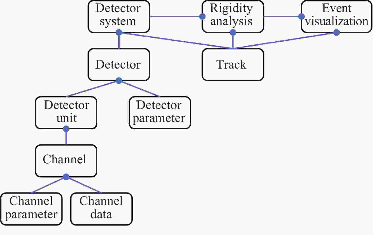
Figure 2. (color online) The class hierarchy in ANAETF.
-
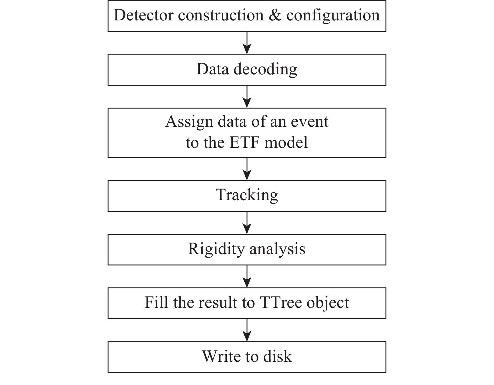
The data processing flow is illustrated in Fig. 3. Once initiated, the main program would instantiate a model of ETF (ETF model) consisting of a hierarchy of detectors of various levels, and ultimately, the readout channels, as mentioned before. Binary raw data are decoded and written in ROOT[15] TTree objects (treeData) with each entry being a hit channel. Adjacent events are separated by a void channel. Multiple binary raw data files containing data of different parts in ETF detector system may be combined as input to ANAETF. They are decoded independently to separate treeData objects.

Figure 3. The data processing flow in ANAETF.
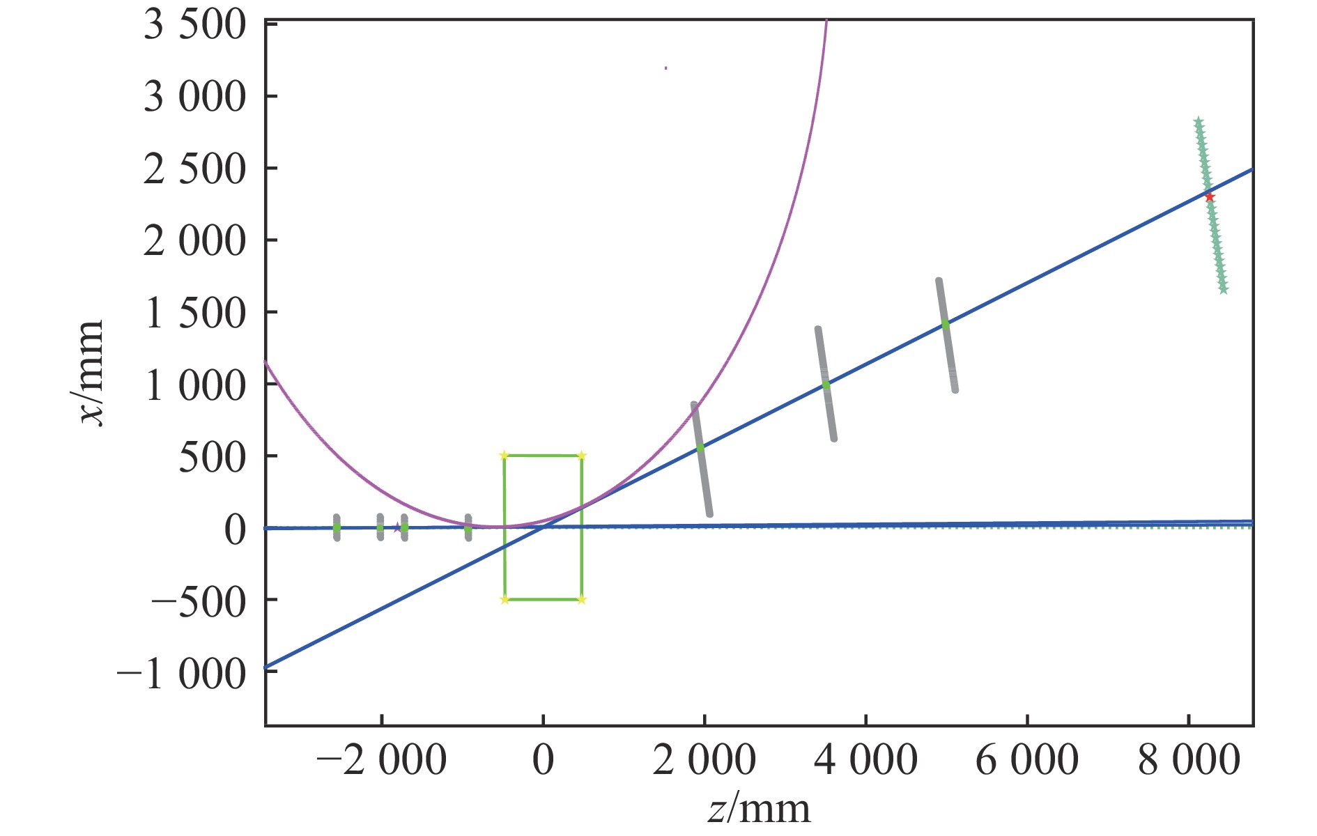
Thereafter while looping over events, ANAETF retrieves all the channels belonging to an event from treeData object(s) to assign to corresponding detector units and channel objects according to their channel IDs. To make the mapping of channel ID to channel feasible, a unique ID (UID) is encoded for each channel according to their position in the detector hierarchy. Once the event is cached in the ETF model, the program filters out the signals that doesn't belong to the trigger-generating particle by setting a time window w.r.t to the trigger time. Particle tracking and rigidity analysis are implemented after the event cache is ready and clean. Optionally, the program visualizes the particle trajectory once the analysis of the event is completed, as Fig. 4 presents. The analysis results are written to a TTree object (treeTrack) for reaction cross section extraction.
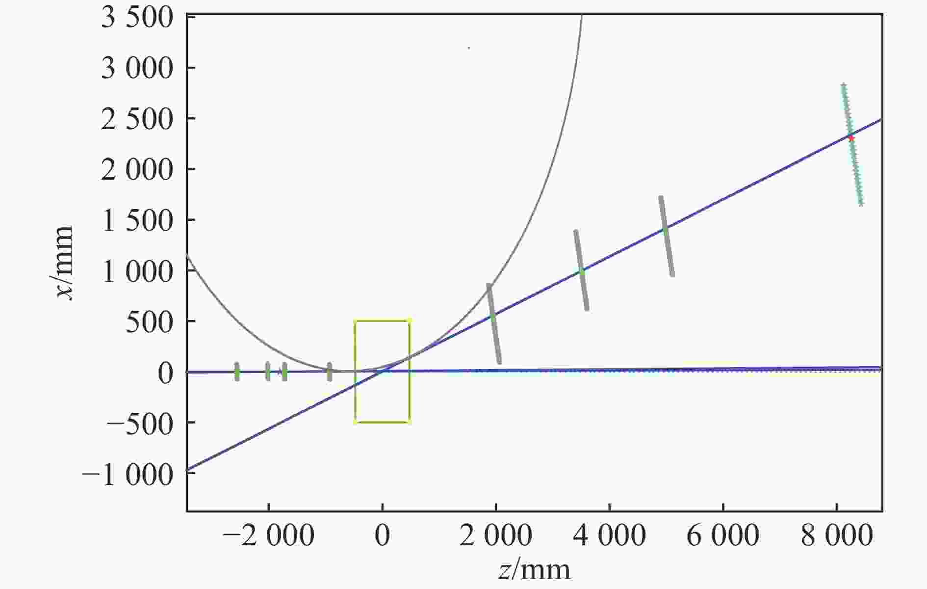
Figure 4. (color online) A snapshot of an event, including the recognized tracks (the blue lines and the magenta arc) and detectors. The green box represents the cavity of the dipole magnet. The green dots in the MWDCs are hit sense wires, while the red dots are for hit strips in TOF Wall.
-
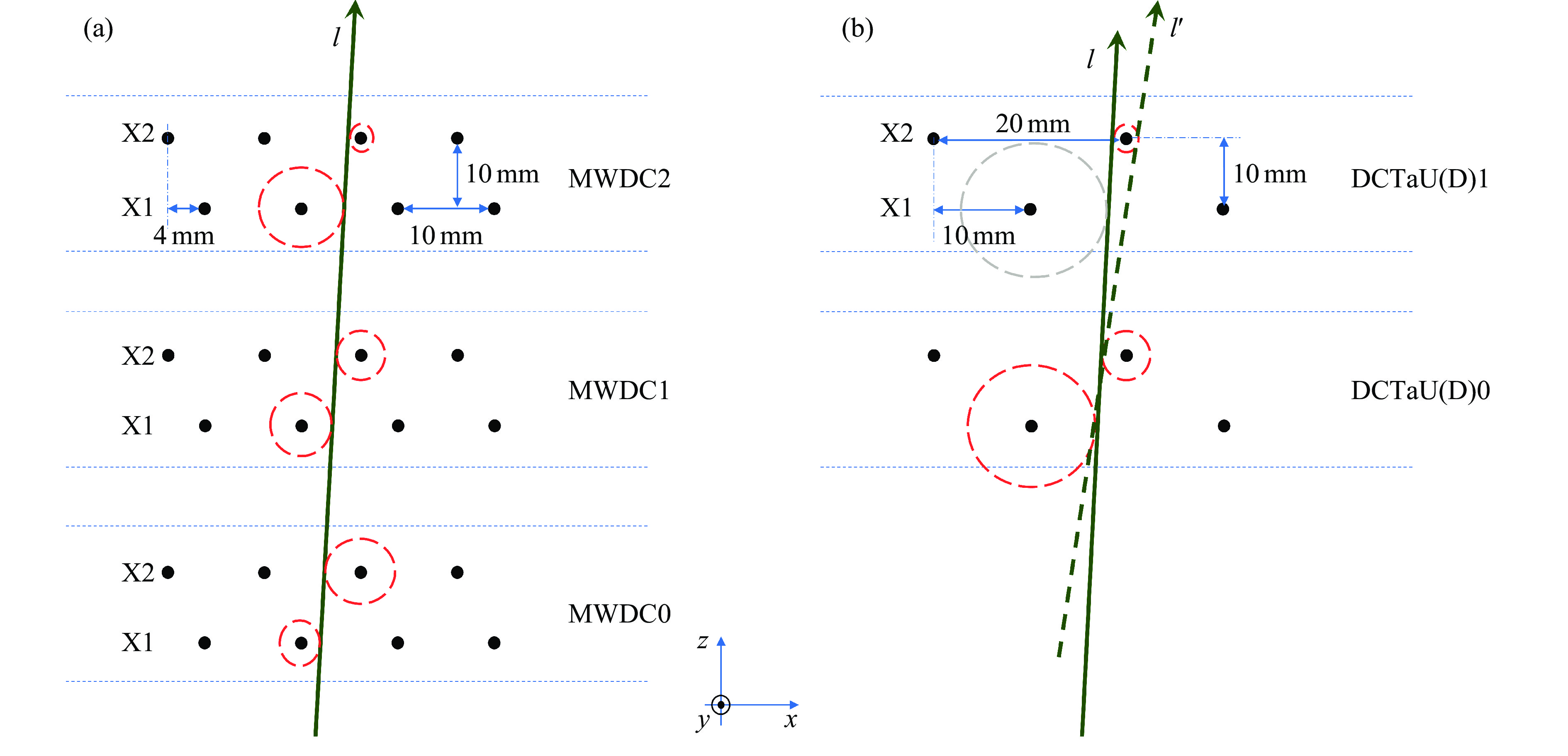
Particle tracks to be reconstructed are all straight tracks outside the magnetic field. The drift chambers in ETF resemble the tracking detectors described in Refs. [16-17]. The tracking algorithm is formulated in full detail in Ref. [1], here we only give a brief description. To begin with, hit sense wires are projected to their normal plane, as is represented by the arrays of dots in Fig. 5 (for X(
$ 0^ \circ $ ) sense wires). A combination of fired sense wires, each from a different sense wire layer, constitutes a track candidate, as exemplified by$ l $ in Fig. 5(a) and$ l $ and$ l^\prime $ in Fig. 5(b). All possible track candidates are put into a two-step procedure: firstly those who are close enough to be considered as belonging to the same particle are tagged as “incompatible”; secondly for each pair of incompatible track candidates, the one with minimal fitting$ \chi^2 $ (the sum of the squares of fitting residues) is preferred as the track of the particle associated with the pair and the other is dropped. This incompatibility check is iterated all along the tracking within an event so as to ensure that no pair of tracks may belong to the same particle. 3-D tracking is implemented afterwards by matching three different track projections from 2-D tracking results to see if they are from the same 3-D track. Note that there are different kinds of track projections that the drift chambers can provide in target zone (X($ 0^ \circ $ ), Y($ 90^ \circ $ )) and downstream the dipole magnet (X($ 0^ \circ $ ), U($ -30^ \circ $ ), V($ +30^ \circ $ )). With the tracking algorithm mentioned above, ANAETF features multiple-track 2-D and 3-D tracking capability.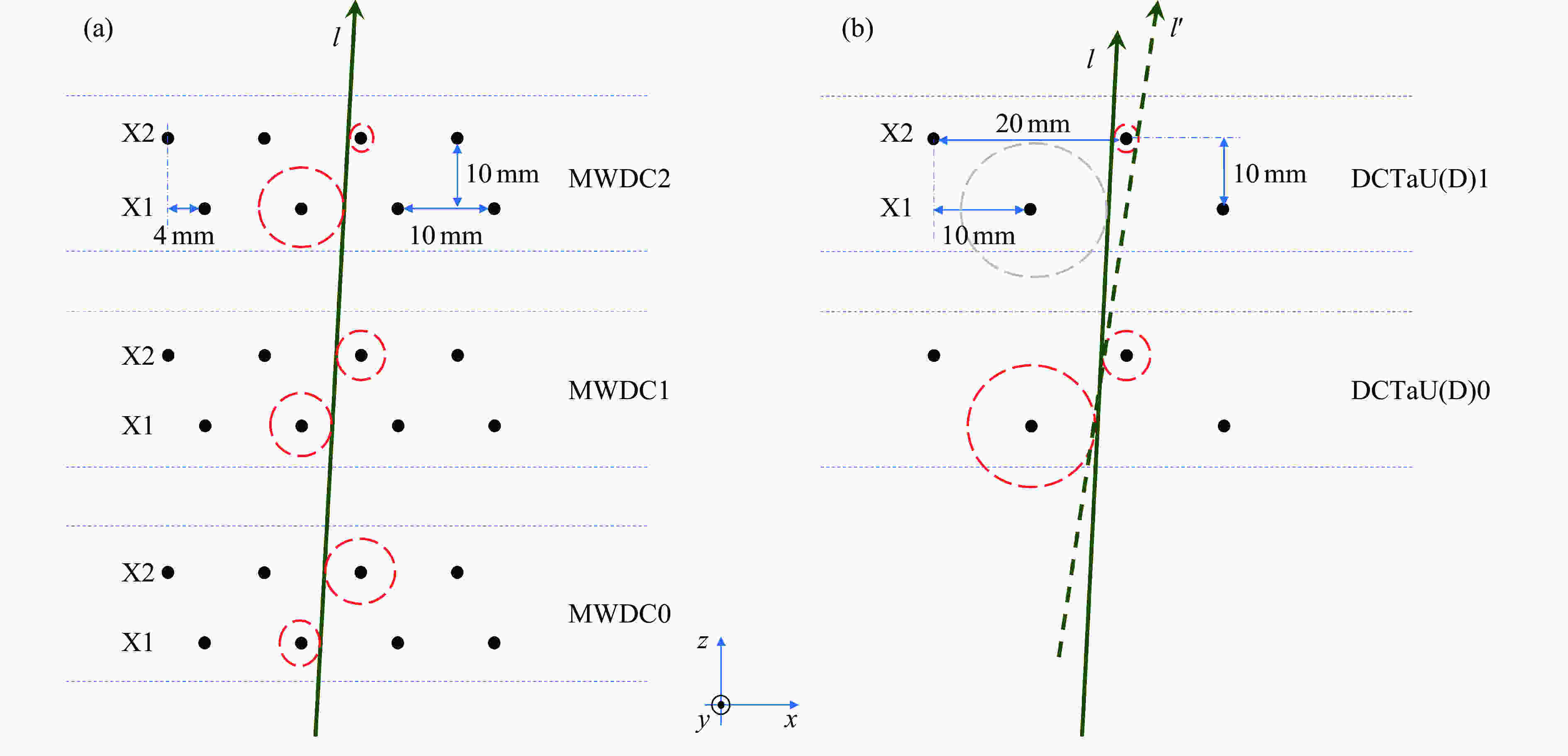
Figure 5. (color online) An illustration (not to scale) of the drift cells and the tracking results of the drift chambers downstream the dipole magnet [Fig. 5(a)] and around the target [Fig. 5(b)]. Dashed circles have their centers at the hit sense wires, and their radii as the drift distances. “Left-right” ambiguity refers to the puzzlement the tracking program may encounter in selecting the left or right side of the drift distance circle for the track to pass by, when information provided by the drift chambers are not sufficient, e.g., when one of the hit drift cells is not fired [the grey circle in Fig. 5(b)].
Progress has been made to the tracking algorithm since Ref. [1]. With
$ 3\!\times\!2 $ X sense wire layers (80 sense wires per layer), the drift chamber array downstream the dipole magnet has tracking efficiency$ \sim\! 100\% $ for carbon isotopes, and seldom encounters the so-called “left-right” ambiguity[1](see Fig. 5). By comparison, drift chamber array DCTaU(D) has only$ 2\!\times\!2 $ X sense wire layers (7 sense wires per layer), resulting in a lower tracking efficiency (averaged at 96% for carbon isotopes), and the “left-right” ambiguity occurring at a higher rate. It can be told from Fig. 5(b) that it's difficult to choose track$ l $ against$ l^\prime $ only by using$ \chi^2 $ minimization, if there's one drift cell passed by a particle yet not fired. The high particle flux around the target makes situation even worse, resulting in high hit multiplicities and increasing tracking errors. Extra information besides the drift chamber array are found to be of help in improving the tracking quality around the target. By taking advantage of the consistency of the tracks on both sides of the target (preTaTrk and postTaTrk), and downstream the dipole magnet (postMagTrk), the discrepancy ($ dx_{\rm{Ta}} $ ) between target hit points extrapolated from preTaTrk and postTaTrk are included quadratically into the fitting$ \chi^2 $ in a joint tracking of preTaTrk and postTaTrk. With$ x_2 $ denoted as the points where particle exits the magnetic field, also quadratically included in the fitting$ \chi^2 $ is the discrepancy ($ dx_2 $ ) between$ x_2 $ extrapolated from postMagTrk and that from particle trajectory (the arc in Fig. 4) in the magnetic field, which starts from postTaTrk (the arc is tangent to postTaTrk).$ dx_{\rm{Ta}} $ and$ dx_2 $ only intervene in solving “left-right” ambiguity during the tracking process to avoid manipulating data, so that after the “left-right” ambiguity is solved, the fitting$ \chi^2 $ minimization is implemented independent of the information from other tracks. Appreciable improvement has been achieved in the PID spectrum with the help of$ dx_{\rm{Ta}} $ and$ dx_2 $ . -
The program adopts a naive approach to deduce magnetic rigidity from the tracks entering and exiting the magnetic field, i.e. assuming a uniform magnetic field, neglecting fringe field and transverse field components (
$ B_x $ and$ B_z $ )[2]. Using the slope and the intercept of the track entering (postTaTrk) and the slope of the track exiting (postMagTrk) the magnetic field, an analytical solution to the arc matching the two tracks at both ends exists. The radius$ \rho $ of the arc is extracted to calculate particle$ A/Z $ ($ aoz $ ) following the equation$$ B\rho\propto poz = aoz\cdot\beta\gamma, $$ (1) where
$ \gamma $ is the Lorentz factor,$ poz $ =$ p/Z $ , and$ \beta $ is the particle velocity. The effective thickness (along neutral beam direction, i.e,$ z $ -direction) of the uniform magnetic field is calibrated to give the correct$ aoz $ values. Refined method solving particle's equation of motion in realistic nonuniform magnetic field numerically with a 4th-order Runge-Kutta (RK) method has shown no competitiveness over current one in terms of magnetic rigidity resolution. In fact, while the two methods turn out to give no discernible difference in PID resolutions in the analysis of experiment or simulation data, the RK method is more time-consuming. The$ aoz $ resolution is found to be dominated by the contribution from magnetic rigidity resolution, which originates from the spatial resolution of the drift chambers. As a result, the mathematical advantage of the RK method may have vanished compared with the PID method using uniform magnetic field. More details are included in Ref. [2]. -
The reaction cross section for reaction channel
$ i $ is calculated according to formula[18]:$$ \sigma_i = \frac{\Delta N_i}{N_0 t \epsilon}, $$ (2) where
$ \Delta N_i $ is the objective residue count,$ N_0 $ the incident particle count,$ t $ the target nucleus density per area, and$ \epsilon $ the compensation coefficient for detecting efficiency, geometrical acceptance and target thickness effect.$ \sigma_i $ from reactions other than in the reaction target is calculated from target-out runs and subtracted.The incident particles are selected so that they pass through the sensitive areas of all the detectors along the flight path and within the reaction target. Particles between two sequential triggers are counted by pileup rejection circuits to identify events that may cause signal pileup in MUSICs. Energy loss measured by MUSIC0 exhibits appreciable position dependence, where a correction has been introduced accordingly.
The detecting efficiency
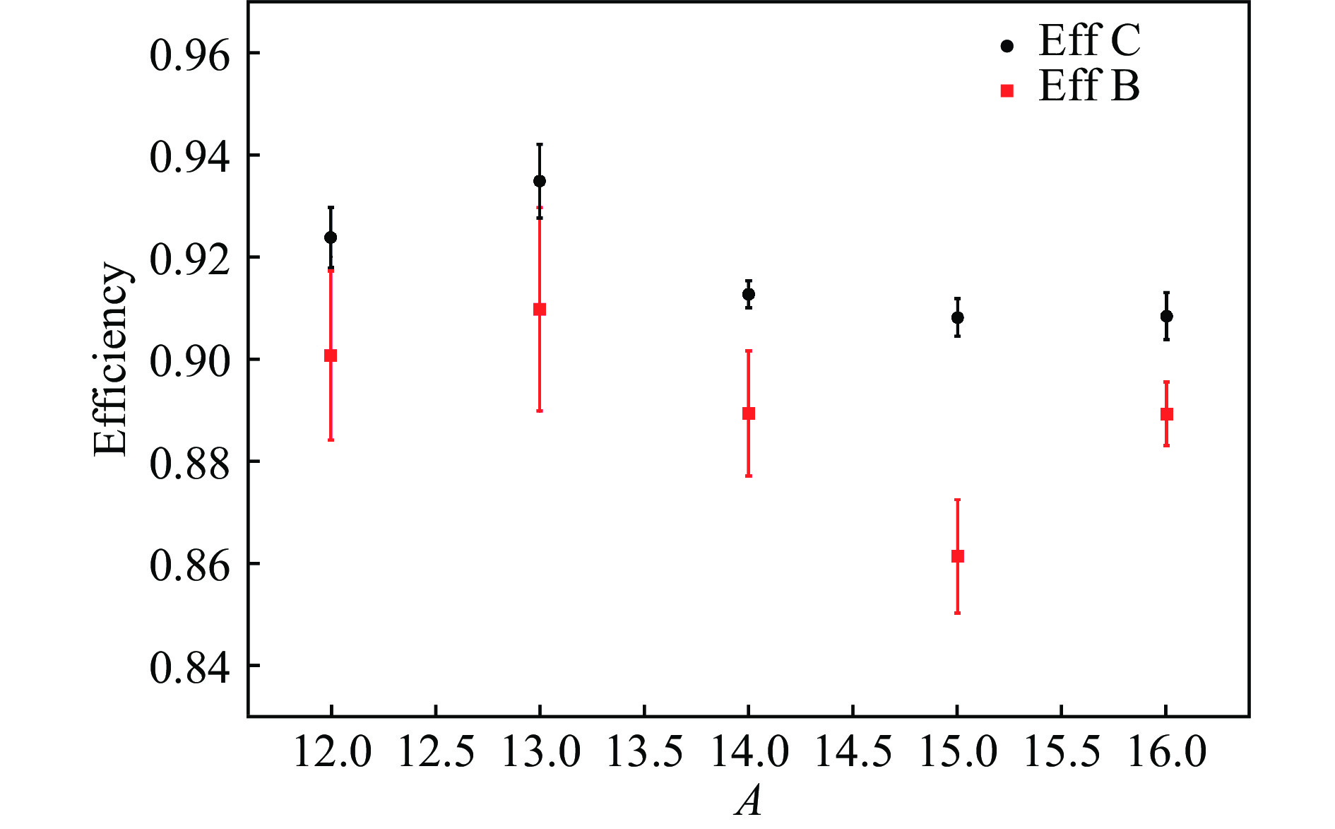
$ \epsilon_{\rm{d}} $ for reaction residues is defined as the probability that a particle falling within the geometrical acceptance of the detecting system get successfully PIDed, i.e. its A and Z identified by the program. Following this definition, as a matter of convenience and simplicity,$ \epsilon_{\rm{d}} $ is calculated in target-out runs as the ratio of the number of successfully PIDed particles to that of incident particles (the PIDed particles and the incident particles are from the same experiment data file for a certain calculation of$ \epsilon_{\rm{d}} $ ). As such,$ \epsilon_{\rm{d}} $ includes contributions from particle reaction loss along the flight path and detecting loss caused by “dead” zones of the gaps between TOF Wall strips. Detecting efficiencies thus calculated for different residues at around 240 MeV/u in ETF are listed in Fig. 6. As is expected,$ \epsilon_{\rm{d}} $ is indifferent to neutron numbers, but shows a slight positive dependence on particle charge, and may vary along experiment runs with the fluctuation of the detectors' working conditions. We note that detecting efficiency is not only determined by detectors, but directly affected by the PID ability of the data analysis program. It can be told from Fig. 6 that$ \epsilon_{\rm{d}} $ for carbon and boron residues are$ \sim 91$ % and$ \sim 88$ % respectively.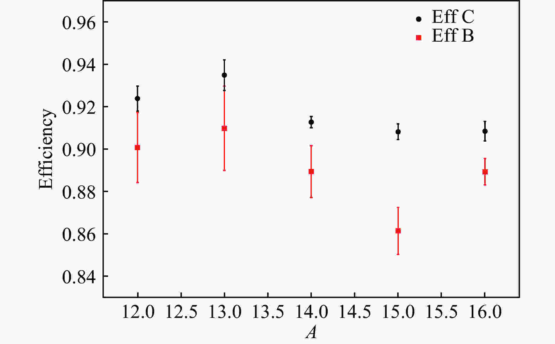
Figure 6. (color online) Detecting efficiencies for carbon and boron residues in ETF at around 240 MeV/u.
Target-thickness effect refers to the cross section loss caused by reaction loss of the incident particles and the objective residues inside the reaction target, and is represented by a compensation coefficient
$ \epsilon_{\rm{SV}} $ calculated as[18]$$ \epsilon_{\rm{SV}} = {\rm e}^{-\sigma_{\rm{I}} t}, $$ (3) where
$ t $ has the same definition as in Eq. (2) and$ \sigma_{\rm{I}} $ is the interaction cross section[19] for the incident nucleus in the target (“SV” stands for “survival”). Practically,$ \sigma_{\rm{I}} $ is calculated from the same experiment data. Since the calculation of$ \sigma_{\rm{I}} $ needs itself as input, it is iterated to a convergence.Geometrical efficiency
$ \epsilon_{\rm{g}} $ is estimated assuming a Gaussian horizontal distribution of reaction residues on TOF Wall. The patch missing from a peak is delineated by fitting the incomplete peak with a Gaussian, and compensated for by its shape. Due to the large size of the MWDCs and TOF Wall downstream the dipole magnet, usually the acceptance for one-nucleon-removal products is 100% and better than 90% for -2n product while the unreacted beam is tuned to the center of TOF Wall. -
Running in normal mode (2-D tracking with least squares method), ANAETF takes about 4.1 s to analyze each 1 000 events in a laptop equipped with Intel(R) Core(TM) i7-8550U CPU @1.80 GHz and 8 GB RAM, corresponding to 14 min for analysis of a typical data file containing 200 000 events. Fig. 7 shows the PID spectrum of the reaction residues produced by 240 MeV/u 12C impinging on a carbon target, where the particle atomic number
$ Z $ is calculated via$ \Delta E\propto Z^2/\beta^2 $ , and$ aoz $ extracted following Eq. (1). The extracted cross sections for -n, -p, -2n and -np processes are compared with results from Ref. [20] for 12C incident at 250, 1 050 and 2 100 MeV/u in Table 1. Systematic errors from different labs considered, our results agree well with theirs.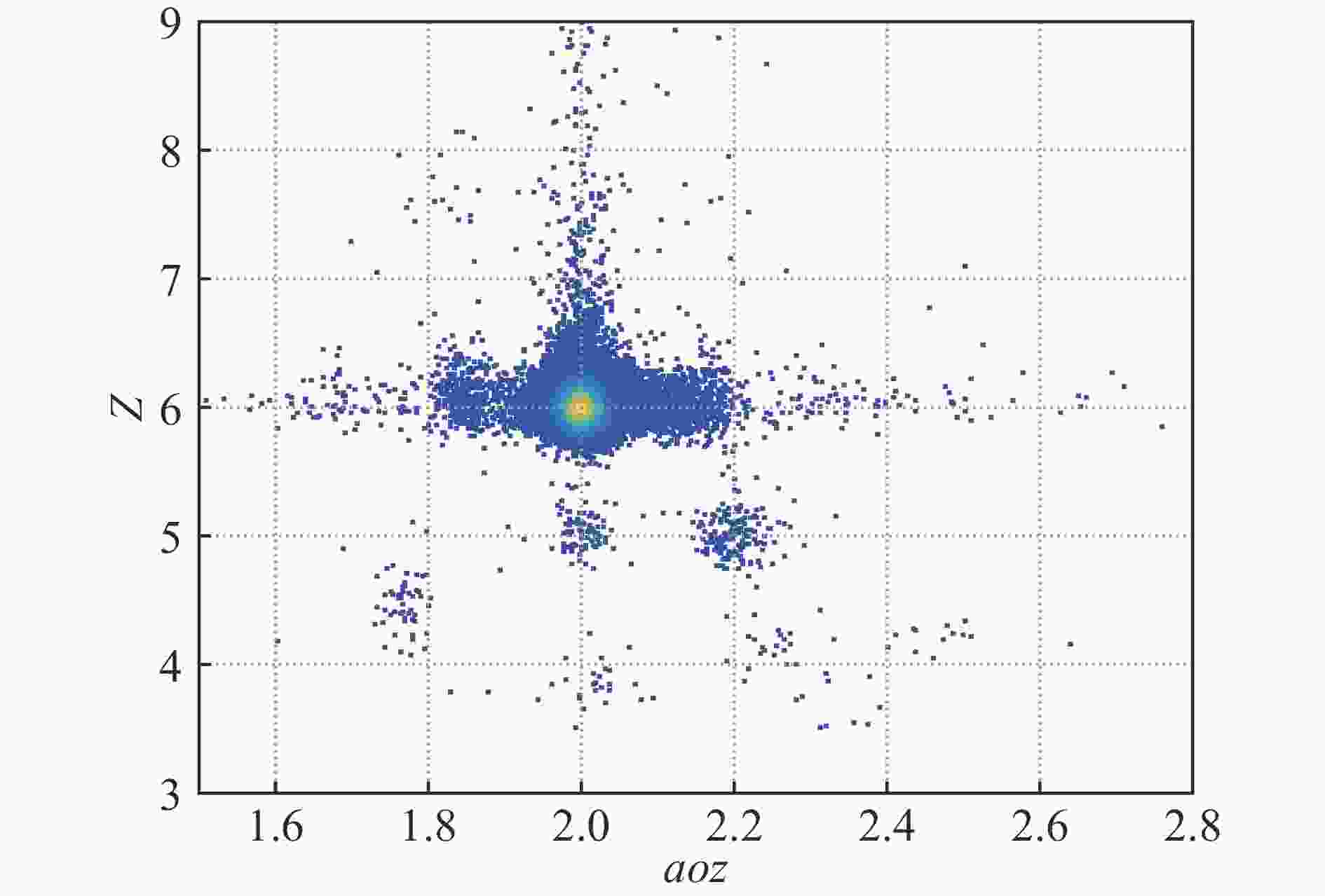
Figure 7. (color online) The PID spectrum of fragments from reaction of 240 MeV/u 12C impinging on a carbon target. The tail to the right of the unreacted 12C corresponds to particles skimming over the edge of TOF Wall strips, resulting in delayed timing (probability ~2%).
Table 1. Cross sections of 12C incident at different energies.
mb Residue 240 MeV/ua 250 MeV/ub 1 050 MeV/ub 2 100 MeV/ub 11C 60.51(11.08) 55.97(4.06) 44.70(2.80) 46.50(2.30) 10C 0.99(5.24) 5.33(0.81) 4.44(0.24) 4.11(0.22) 11B 62.37(5.67) 65.61(2.55) 48.60(2.40) 53.80(2.70) 10B 35.29(4.70) 47.50(2.42) 27.90(2.20) 35.10(3.40) a This work.
b Ref. [20]. -
ETF is established for reaction studies using intermediate and high energy stable beams and RIBs, for which a large data analysis framework (ANAETF) is developed. ANAETF adopts OO-programming for the modelling of ETF and interfaces ROOT so as to be easily maintainable and extensible. The program has achieved satisfying performance in particle identification and cross section extration with acceptable computing speed[21-22].
Acknowledgement The authors would like to thank the HIRFL-CSR accelerator staff for preparing the primary and secondary beams.
Data Analysis Framework for Radioactive Ion Beam Experiments at the External Target Facility of HIRFL-CSR
-
摘要: 开发了HIRFL-CSR外靶实验装置的大型数据分析程序(ANAETF),并成功应用于核物理实验数据分析。详细阐述了该程序中的数据分析流程、漂移室寻迹算法、粒子鉴别方法和反应截面提取技术。利用本程序分析了240 MeV/u能量下12C次级束流打碳靶的实验数据,实现了清楚的碳和硼剩余核的粒子鉴别,总探测效率达到 ~90%,本工作提取的反应截面与已有的实验结果符合较好。Abstract: ANAETF, a large data analysis framework for the External Target Facility (ETF) of HIRFL-CSR, has been developed and successfully used for data analysis in radioactive ion beam experiments. This paper covers the flow of data processing in the program, the general tracking algorithm for the drift chambers, the particle identification (PID) approach, and the techniques for extraction of reaction cross sections. The program achieves total detecting efficiencies of around ~90% and gives clear PID spectrum for carbon and beryllium fragments produced from the reaction of 240 MeV/u 12C secondary beams on a carbon target. The obtained cross sections are consistent with the previously reported experimental results.
-
Figure 4. (color online) A snapshot of an event, including the recognized tracks (the blue lines and the magenta arc) and detectors. The green box represents the cavity of the dipole magnet. The green dots in the MWDCs are hit sense wires, while the red dots are for hit strips in TOF Wall.
Figure 5. (color online) An illustration (not to scale) of the drift cells and the tracking results of the drift chambers downstream the dipole magnet [Fig. 5(a)] and around the target [Fig. 5(b)]. Dashed circles have their centers at the hit sense wires, and their radii as the drift distances. “Left-right” ambiguity refers to the puzzlement the tracking program may encounter in selecting the left or right side of the drift distance circle for the track to pass by, when information provided by the drift chambers are not sufficient, e.g., when one of the hit drift cells is not fired [the grey circle in Fig. 5(b)].
Figure 6. (color online) Detecting efficiencies for carbon and boron residues in ETF at around 240 MeV/u.
Figure 7. (color online) The PID spectrum of fragments from reaction of 240 MeV/u 12C impinging on a carbon target. The tail to the right of the unreacted 12C corresponds to particles skimming over the edge of TOF Wall strips, resulting in delayed timing (probability ~2%).
Table 1. Cross sections of 12C incident at different energies.
mb Residue 240 MeV/ua 250 MeV/ub 1 050 MeV/ub 2 100 MeV/ub 11C 60.51(11.08) 55.97(4.06) 44.70(2.80) 46.50(2.30) 10C 0.99(5.24) 5.33(0.81) 4.44(0.24) 4.11(0.22) 11B 62.37(5.67) 65.61(2.55) 48.60(2.40) 53.80(2.70) 10B 35.29(4.70) 47.50(2.42) 27.90(2.20) 35.10(3.40) a This work.
b Ref. [20]. 下载: 导出CSV
-
[1] SUN Y Z, SUN Z Y, WANG S T, et al. Nucl Instr and Meth A, 2018, 894: 72. doi: 10.1016/j.nima.2018.03.044 [2] Sun Y Z, SUN Z Y, WANG S T, et al. Nucl Instr and Meth A, 2019, 927: 390. doi: 10.1016/j.nima.2019.02.067 [3] CHENG Z H, YU Y H, SUN Z Y, et al. Nuclear Physics Review, 2019, 36(3): 343. (in Chinese) doi: 10.11804/NuclPhysRev.36.03.343 [4] FANG F, YUE K, SUN Z Y, et al. Nuclear Physics Review, 2017, 34(2): 184. (in Chinese) doi: 10.11804/NuclPhysRev.34.02.184 [5] YAN D, YUE K, SUN Z Y, et al. Nuclear Physics Review, 2016, 33(4): 455. (in Chinese) doi: 10.11804/NuclPhysRev.33.04.455 [6] LU W, CHEN Z Q, KONG J, et al. Nuclear Physics Review, 2011, 28(4): 464. (in Chinese) doi: 10.11804/NuclPhysRev.28.04.464 [7] YUE K, XU H S, LIANG J J, et al. Nuclear Physics Review, 2010, 27(4): 445. (in Chinese) doi: 10.11804/NuclPhysRev.27.04.445 [8] XIA J W, ZHAN W L, WEI B W, et al. Nucl Instr and Meth A, 2002, 488: 11. doi: 10.1016/S0168-9002(02)00475-8 [9] TANG S W, DUAN L M, SUN Z Y, et al. Nuclear Physics Review, 2012, 29(1): 072. (in Chinese) doi: 10.11804/NuclPhysRev.29.01.072 [10] SUN B H, ZHAO J W, ZHANG X H, et al. Sci Bull, 2018, 63: 78. doi: 10.1016/j.scib.2017.12.005 [11] SUN Y, SUN Z Y, YU Y H, et al. Nucl Instr and Meth A, 2018, 893: 68. doi: 10.1016/j.nima.2018.03.030 [12] ZHANG X H, TANG S W, MA P, et al. Nucl Instr and Meth A, 2015, 795: 389. doi: 10.1016/j.nima.2015.06.022 [13] KIMURA K, IZUMIKAWA T, KOYAMA R, et al. Nucl Instr and Meth A, 2005, 538: 608. doi: 10.1016/j.nima.2004.08.100 [14] ANAETF, Data Analysis Framework for the External Target Facility, HIRFL-CSR[EB/OL].[2020-11-24]. https://github.com/asiarabbit/BINGER.git. [15] ROOT: Analyzing Petabytes of Data, Scientically[EB/OL].[2020-11-24]. https://root.cern.ch. [16] YI H, ZHANG Z, XIAO Z G, et al. Chin Phys C, 2014, 38: 126002. doi: 10.1088/1674-1137/38/12/126002 [17] KOBAYASHI T, CHIGA N, ISOBE T, et al. Nucl Instr and Meth B, 2013, 317: 294. doi: 10.1016/j.nimb.2013.05.089 [18] SUN Y Z. Study of Single Proton Knockout from 16C[D]. Lanzhou: Institute of Modern Physics, Chinese Academy of Sciences, 2019. (in Chinese) [19] KOHAMA A, IIDA K, OYAMATSU K. Phys Rev C, 2008, 78: 061601. doi: 10.1103/PhysRevC.78.061601 [20] KIDD J M, LINDSTROM P J, CRAWFORD H J, et al. Phys Rev C, 1988, 37: 2613. doi: 10.1103/PhysRevC.37.2613 [21] SUN Y Z, WANG S T, SUN Z Y, et al. Phys Rev C, 2019, 99: 024605. doi: 10.1103/PhysRevC.99.024605 [22] ZHAO Y X, SUN Y Z, WANG S T, et al. Phys Rev C, 2019, 100: 044609. doi: 10.1103/PhysRevC.100.044609 -

 点击查看大图

计量
- 文章访问数: 660
- HTML全文浏览量: 133
- PDF下载量: 70
- 被引次数: 0


 甘公网安备 62010202000723号