


-
As a superconducting (SC) proton linear accelerator (linac), the China Accelerator Driven sub-critical System (C-ADS) demo facility is developed in the Institute of Modern Physics, Chinese Academy of Sciences (IMP, CAS), and it accelerates 10 mA proton beam up to 25 MeV, as shown in Table 1[1].
Table 1. C-ADS demo linac parameters.
Parameters Value Unit Particle Proton — Energy 25 MeV Beam current 10 mA Duty factor 100 % Bunch frequency 162.5 MHz The SC section includes 23 SC cavities in 4 cryomodules. The beam energy reaches 2.12 MeV at the exit of RFQ, and the MEBT (Medium Energy Beam Transport) layout is shown in Fig. 1[2], including 7 quadrupoles and 2 bunchers.

Figure 1. (color online) MEBT layout of C-ADS demo linac.
The proton beam is bunched in the RFQ in the linac. For better matching in MEBT and SC accelerating sections, it is important to know beam parameters at the exit of RFQ, especially in the longitudinal phase plane, which is also significant for building a virtual accelerator in simulation code. Beam transverse parameters are measured by wires in the MEBT of the linac. The paper introduces an experiment for measuring the longitudinal emittance and twiss parameters by beam position monitors (BPMs), including theory, simulation, experiment and discussion.
Two bunchers located at the MEBT of the linac and several downstream BPMs are used for the experiment. By adjusting the voltage and phase of the bunchers, signals on BPMs are recorded and analyzed. The recorded BPMs' signals are called SUM-signals and they are relevant to the longitudinal distribution of the beam bunch.
-
For the longitudinal Gaussian distribution beam, current density
$ \lambda(z) $ is associated with the position$ z $ [3]:$$ \lambda(z) = \frac{q \cdot N}{\sigma_{z} \cdot \sqrt{2 \pi}} \cdot {\rm{e}}^{-\frac{z^{2}}{2 \cdot \sigma_{z}^{2}}}, $$ (1) where
$ \sigma_{z} $ is the longitudinal RMS size of the bunch,$ q $ is the charge of each particle, and$ N $ is the number of particles in the bunch. The current density in the time domain is$ \lambda(t) = \lambda(z)|_{z = \beta ct} \cdot \beta c $ , where$ \beta c $ is the velocity of the bunch, then the SUM-signal of BPM is the integral value of Fourier transform of$ \lambda(t) $ [3]:$$ \begin{split} SUM =& A_{0} \cdot \int\nolimits_{-\infty}^{\infty} {\rm{e}}^{{\rm{i}}\omega t} \cdot \frac{q \cdot N}{\sigma_{z} \cdot \sqrt{2 \pi}} \cdot {\rm{e}}^{-\frac{(\beta c t)^{2}}{2 \sigma_{z}^{2}}} \cdot \beta c \cdot {\rm{d}}t \\ =& A_{0} \cdot \frac{I_{0}}{f_{0}} \cdot {\rm{e}}^{-\frac{2 \pi^{2}}{(\beta \lambda)^{2}}\cdot\sigma_{z}^{2}}, \end{split} $$ (2) where
$ A_{0} $ is the BPM's amplification coefficient,$ I_{0} $ is the current of the beam,$ f_{0} $ is the bunch frequency, and$ \lambda = \frac{c}{f_{0}} $ .The transfer matrix in the longitudinal phase plane is[4]:
$$ \left[ {\begin{array}{*{20}{c}} {{z_1}}\\ {z_1^\prime } \end{array}} \right] = \left[ {\begin{array}{*{20}{l}} {{m_{11}}}&{{m_{12}}}\\ {{m_{21}}}&{{m_{22}}} \end{array}} \right]\left[ {\begin{array}{*{20}{c}} {{z_0}}\\ {z_0^{\prime} } \end{array}} \right], $$ (3) where
$ z $ and$ z' $ are the RMS beam size and RMS angular divergence in the longitudinal plane respectively, and the subscript index 0 and 1 indicate the initial state and the final state. The expression for the squared RMS beam size$ \left\langle z_{1}^{2}\right\rangle $ is related with the initial RMS beam size and angular divergence:$$\begin{split} \left\langle z_{1}^{2}\right\rangle =& m_{11}^{2}\cdot\left\langle z_{0}^{2}\right\rangle+2 m_{11}m_{12}\cdot\left\langle z_{0} z_{0}^{\prime}\right\rangle+m_{12}^{2}\cdot\left\langle z_{0}^{\prime 2}\right\rangle \end{split}.$$ (4) Then, the squared RMS beam sizes
$ \left\langle z_{i}^{2}\right\rangle $ in different transfer matrix are:$ \left[ {\begin{array}{*{20}{c}} {\left\langle {z_1^2} \right\rangle }\\ {\left\langle {z_2^2} \right\rangle }\\ \ldots \\ {\left\langle {z_n^2} \right\rangle } \end{array}} \right] = \left[ {\begin{array}{*{20}{c}} {{{\left( {m_{11}^{(1)}} \right)}^2}}&{2m_{11}^{(1)}m_{12}^{(1)}}&{{{\left( {m_{12}^{(1)}} \right)}^2}}\\ {{{\left( {m_{11}^{(2)}} \right)}^2}}&{2m_{11}^{(2)}m_{12}^{(2)}}&{{{\left( {m_{12}^{(2)}} \right)}^2}}\\ \cdots & \cdots & \cdots \\ {{{\left( {m_{11}^{(n)}} \right)}^2}}&{2m_{11}^{(n)}m_{12}^{(n)}}&{{{\left( {m_{12}^{(n)}} \right)}^2}} \end{array}} \right]\left[ {\begin{array}{*{20}{c}} {\left\langle {z_0^2} \right\rangle }\\ {\left\langle {{z_0}z_0^\prime } \right\rangle }\\ {\left\langle {z_0^{\prime 2}} \right\rangle } \end{array}} \right], $ (5) From Eq. (2) and (5), the relationship between BPM signals and the initial beam parameters is:
$$ \begin{array}{*{20}{l}} {\left[ {\begin{array}{*{20}{c}} {A \cdot \ln {{\left( {SUM} \right)}^{(1)}} - A \cdot \ln \left( {{A_0} \cdot \frac{{{I_0}}}{{{f_0}}}} \right)}\\ {A \cdot \ln {{\left( {SUM} \right)}^{(2)}} - A \cdot \ln \left( {{A_0} \cdot \frac{{{I_0}}}{{{f_0}}}} \right)}\\ \cdots \\ {A \cdot \ln {{\left( {SUM} \right)}^{(n)}} - A \cdot \ln \left( {{A_0} \cdot \frac{{{I_0}}}{{{f_0}}}} \right)} \end{array}} \right] = } {\left[ {\begin{array}{*{20}{c}} {{{\left( {m_{11}^{(1)}} \right)}^2}}&{2m_{11}^{(1)}m_{12}^{(1)}}&{{{\left( {m_{12}^{(1)}} \right)}^2}}\\ {{{\left( {m_{11}^{(2)}} \right)}^2}}&{2m_{11}^{(2)}m_{12}^{(2)}}&{{{\left( {m_{12}^{(2)}} \right)}^2}}\\ \cdots & \cdots & \cdots \\ {{{\left( {m_{11}^{(n)}} \right)}^2}}&{2m_{11}^{(n)}m_{12}^{(n)}}&{{{\left( {m_{12}^{(n)}} \right)}^2}} \end{array}} \right]\left[ {\begin{array}{*{20}{c}} {\left\langle {z_0^2} \right\rangle }\\ {\left\langle {{z_0}z_0^\prime } \right\rangle }\\ {\left\langle {z_0^{\prime 2}} \right\rangle } \end{array}} \right]{\mkern 1mu} ,} \end{array}$$ (6) where
$ A = -\frac{(\beta \lambda)^{2}}{2 \pi^{2}} = -\frac{\left(\beta c / f_{0}\right)^{2}}{2 \pi^{2}} $ , and finally we get$$\begin{array}{*{20}{l}} {\left[ {\begin{array}{*{20}{c}} {{{\left( {m_{11}^{(1)}} \right)}^2}}&{2m_{11}^{(1)}m_{12}^{(1)}}&{{{\left( {m_{12}^{(1)}} \right)}^2}}&1\\ {{{\left( {m_{11}^{(2)}} \right)}^2}}&{2m_{11}^{(2)}m_{12}^{(2)}}&{{{\left( {m_{12}^{(2)}} \right)}^2}}&1\\ \cdots & \cdots & \cdots &{}\\ {{{\left( {m_{11}^{(n)}} \right)}^2}}&{2m_{11}^{(n)}m_{12}^{(n)}}&{{{\left( {m_{12}^{(n)}} \right)}^2}}&1 \end{array}} \right] \cdot } {\left[ {\begin{array}{*{20}{c}} {\left\langle {z_0^2} \right\rangle }\\ {\left\langle {{z_0}z_0^\prime } \right\rangle }\\ {\left\langle {z_0^{\prime 2}} \right\rangle }\\ {A \cdot \ln \left( {{A_0} \cdot \frac{{{I_0}}}{{{f_0}}}} \right)} \end{array}} \right] = \left[ {\begin{array}{*{20}{c}} {A \cdot \ln {{\left( {SUM} \right)}^{(1)}}}\\ {A \cdot \ln {{\left( {SUM} \right)}^{(2)}}}\\ \cdots \\ {A \cdot \ln {{\left( {SUM} \right)}^{(n)}}} \end{array}} \right]{\mkern 1mu} ,} \end{array}$$ (7) The initial beam information
$ \left\langle z_{0}^{2}\right\rangle $ ,$ \left\langle z_{0}z_{0}^{\prime}\right\rangle $ and$ \left\langle z_{0}^{\prime 2}\right\rangle $ are calculated from Eq. (7) as long as the transfer matrix and the SUM-signals are known, and the initial beam parameters are[5]:$$ \left\{\begin{array}{l} \varepsilon = \sqrt{\left\langle z_{0}^{2}\right\rangle\left\langle z_{0}^{\prime 2}\right\rangle-\left\langle z_{0} z_{0}^{\prime}\right\rangle^{2}} \\ \alpha = -\left\langle z_{0} z_{0}^{\prime}\right\rangle / \varepsilon \\ \beta = \left\langle z_{0}^{2}\right\rangle / \varepsilon \end{array}\right., $$ (8) where
$ \varepsilon $ is the emittance,$ \alpha $ and$ \beta $ are twiss parameters. -
Two bunchers for bunching the beam in the longitudinal plane are installed at the MEBT of C-ADS demo linac, as shown in Fig. 1. According to the simulation results in Toutatis[6], beam parameters at the exit of RFQ are
$ {\varepsilon _{{\rm{Norm,RMS}}}} = 0.297\,8\;{\rm{\pi }} \cdot {\rm{mm}} \cdot {\rm{mrad}} $ ,$ \alpha = -0.254\,5 $ ,$ \beta = 1.775\,4 \ \;{\rm{mm}} /({\rm{\pi}} \cdot {\rm{mrad}}) $ . Based on that, the voltages of the two bunchers are scanned in simulation in TraceWin[7], while keeping the synchronous phase to be at$ -90$ ° or 90° to guarantee that the beam energy is fixed.Fig. 2 shows the relationship between the ratio of
$ SUM $ to$ A_0 \cdot \frac{I_0}{f_0} $ and the RMS phase width$ \sigma_{\varphi} $ in a beam bunch[8]. For reducing system errors, the ratio is kept in the reasonable interval of [0.1, 0.9], and the corresponding bunch RMS phase width should be between [27°, 122°], which is far higher than the nominal case, as shown in the blue frame in Fig. 2.
Figure 2. (color online) Bunch length evaluation.
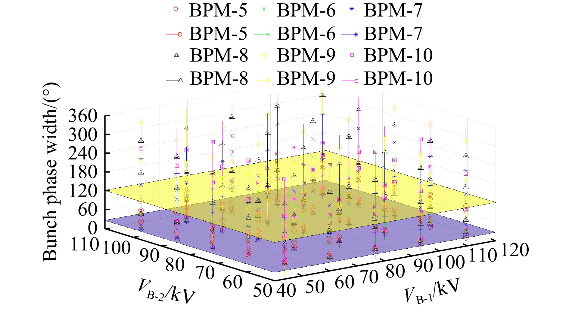
In some cases, the beam in the longitudinal plane is over-bunched or over-debunched beyond the required interval, as shown in Fig. 3, and they should be treated as invalid data, i.e. bunch length selection. For a set of the voltage of the two bunchers, there are four states: B-B, B-DB, DB-B, and DB-DB, here B indicates bunching and DB represents debunching. Considering the amplitude of the two bunchers varying in 5 different stages, there are
$ 5\!\times\!5\times\!4= $ 100 cases in total for each BPM before bunch length selection, and there are about 200 valid cases out of 600 cases for all the 6 BPMs after the selection.
Figure 3. (color online) Bunch length selection. Cases between the two layers ([27°, 122°]) are selected as valid data.
-
Beam parameters are calculated based on Eq. (7) and (8), so the transfer matrix for each case and the corresponding BPM SUM-signals should be calculated and recorded during the experiment. Please note that the term
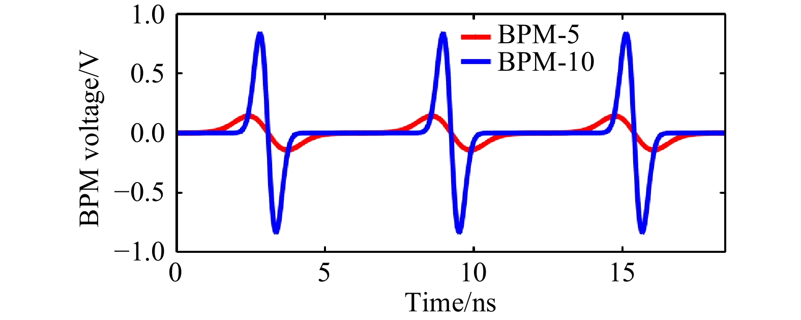
$ A \cdot \ln(A_{0} \cdot \frac{I_{0}}{f_{0}}) $ is unknown.To reduce system errors, 6 BPMs located in the downstream of the MEBT are used. Since the amplification coefficient for each BPM remains unknown before the experiment, the SUM-signals in different BPMs don’t directly reflect the longitudinal distribution of beam bunches. Nevertheless, we still record the SUM-signals rather than the longitudinal bunch profile signals from the view of efficiency on data recording and processing. To show the relationship between the integrated SUM-signals and the longitudinal bunch profiles, the simulated longitudinal bunch profile signals on different BPMs are shown in Fig. 4.
Figure 4. (color online) Simulated longitudinal bunch profile signals on different BPMs. (Pipe diameter and bunch length are different at the two locations).
The experiment was conducted with the probe beam (20 μs@1 Hz) and the beam current is 4.7 mA.
-
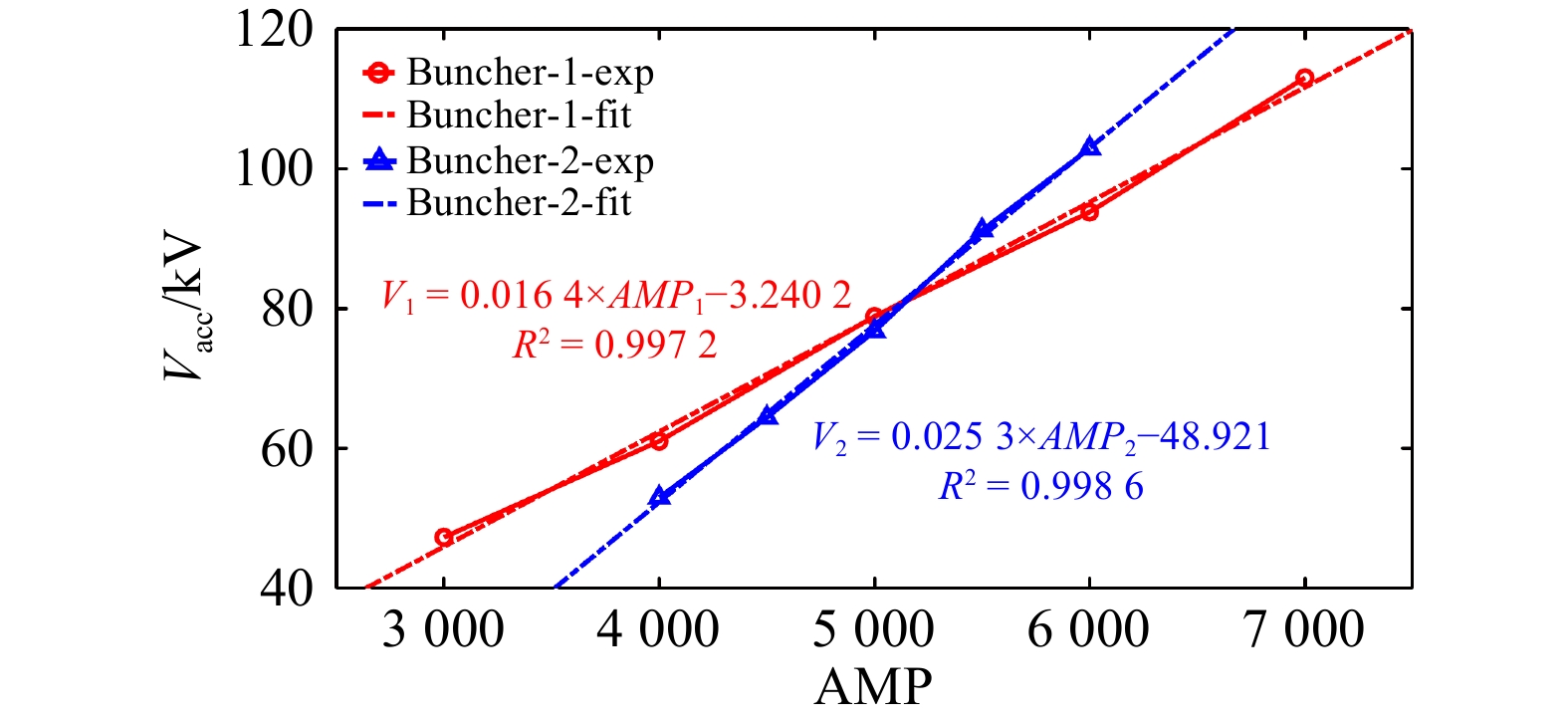
In the experiment, the direct display value of the LLRF (Low Level Radio Frequency) system is the amplitude (AMP) rather than the bunching voltage
$ V_{\rm{acc}} $ . To get$ V_{\rm{acc}} $ , phase scan on different voltages for each buncher is performed and the calibration results are shown in Fig. 5. The calibration verifies the linear relationship between the AMP and the bunching voltage$ V_{\rm{acc}} $ of the two bunchers, and it also provides the relationship between them.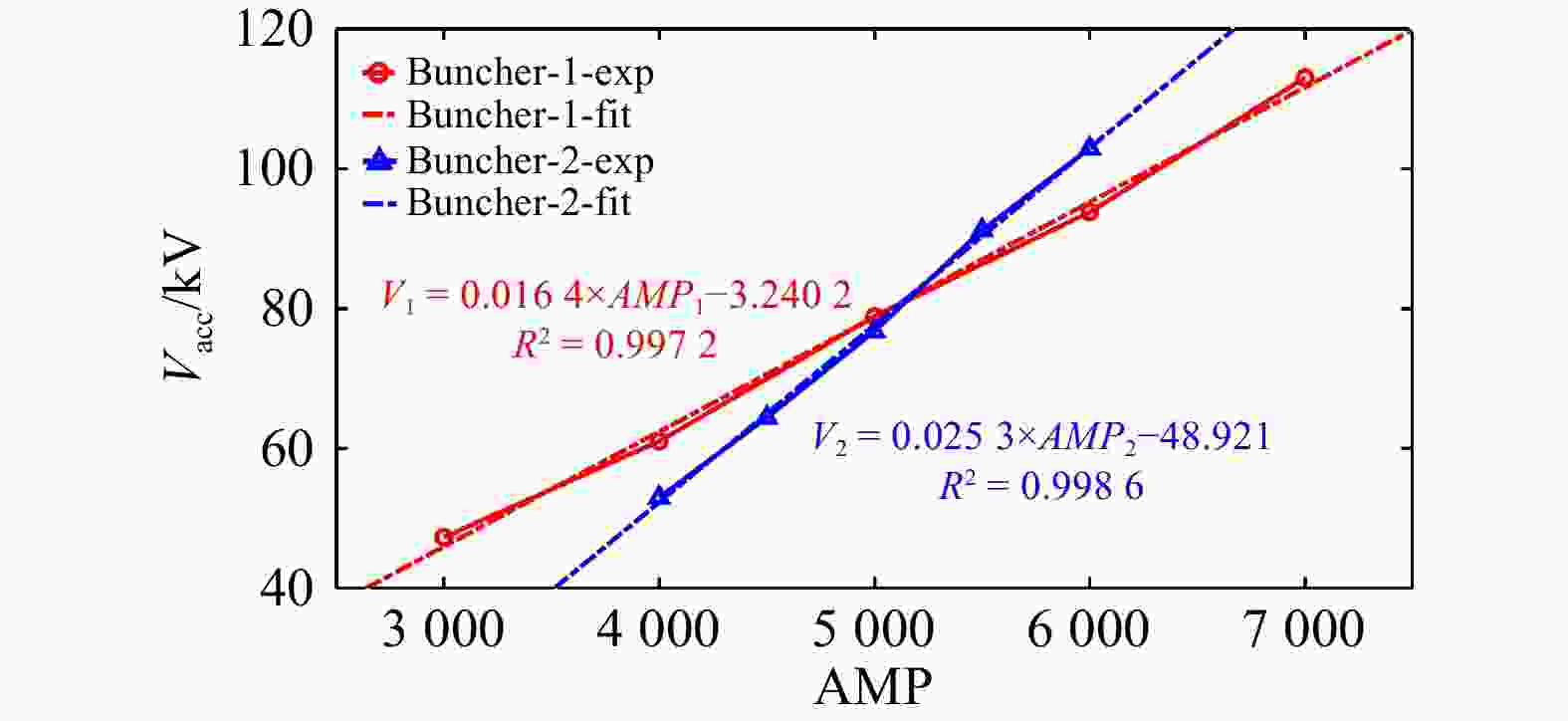
Figure 5. (color online) Buncher amplitude calibration.
The calibration is aimed at getting the right bunching voltage conveniently during the experiment, for further calculation the transfer matrix in Eq. (7) for each case.
To get rid of the influence of different beam energy on BPM signals, the synchronous phases of the bunchers are set to be
$ -90^{\circ} $ or 90°, such that no acceleration in MEBT during the whole experiment, as discussed in Section 3. -
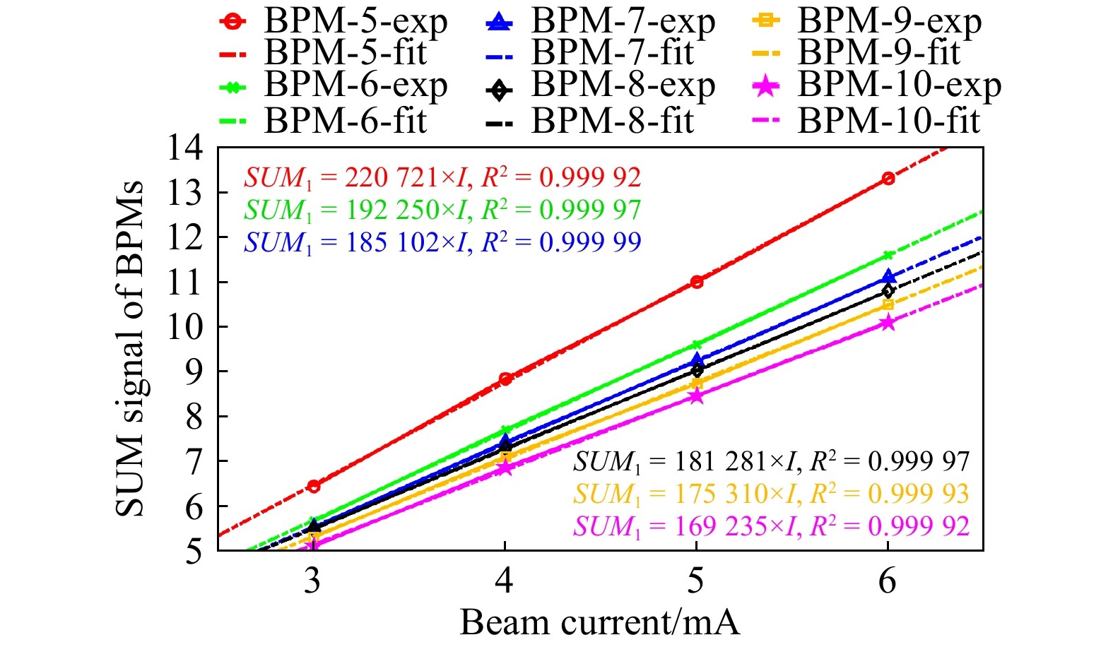
To ensure that the SUM-signals of BPMs are in the linear interval for different beam current, the SUM-current linearity is verified as shown in Fig. 6.
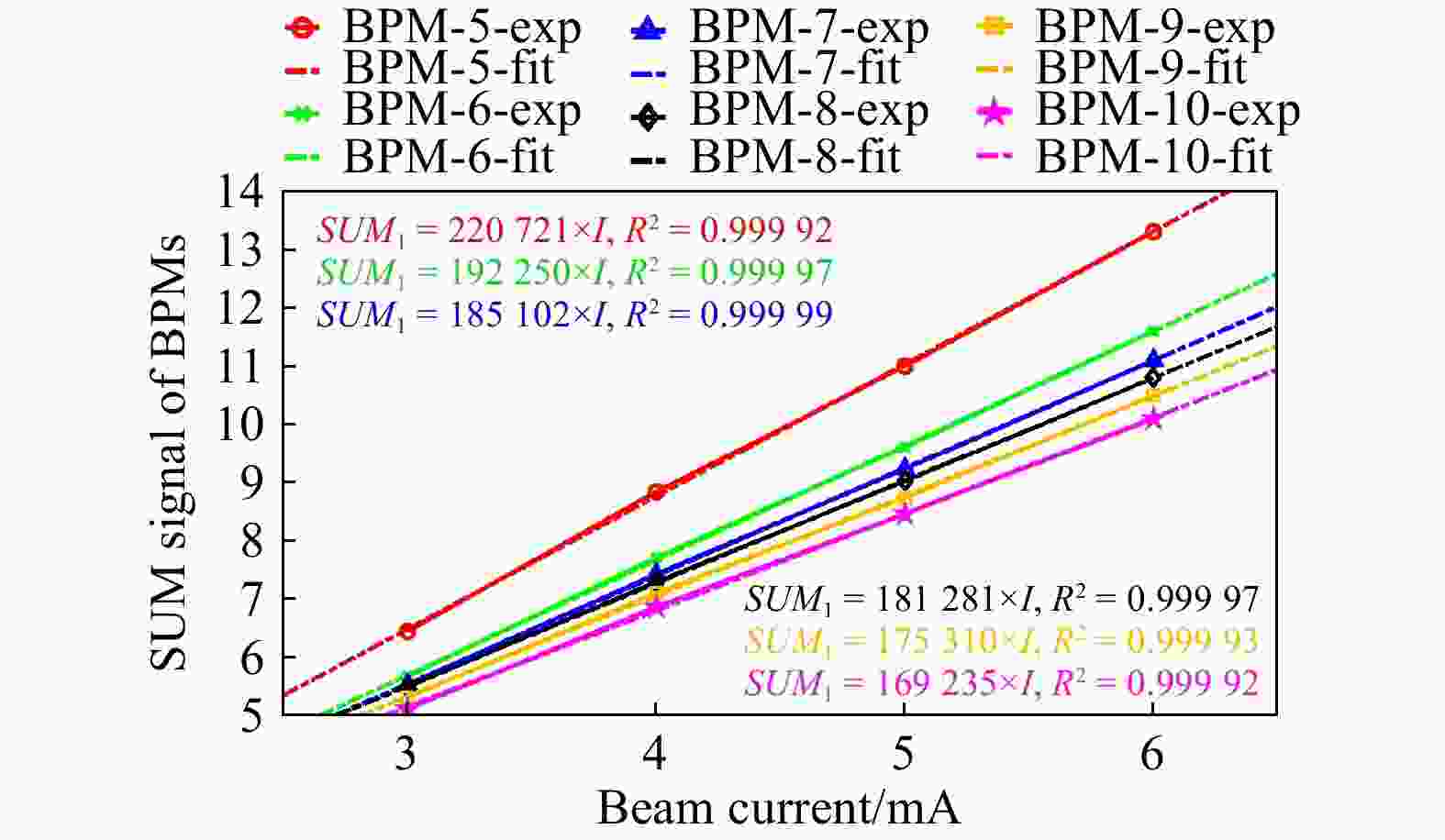
Figure 6. (color online) SUM-current linearity verification for BPMs. (The square of the correlation coefficient for all the BPMs are beyond 0.9999).
-
To form different beam sizes in the longitudinal plane, the voltages of bunchers are scanned, while keeping the synchronous phase stays at
$ -90 $ ° or 90°, and the SUM-signals of downstream BPMs are recorded. The voltage ranges from about 40% of the full value to the maximum. -
According to the simulation, except for bunch length selection, the cases for BPM signals with error beyond 1% should also be deleted.
As has been discussed before, the transfer matrix in Eq. (7) and the corresponding SUM-signals are calculated and recorded during the experiment. We only considered the longitudinal phase plane
$ (z,{\rm{d}}p/p) $ in the matrix and it includes two bunchers, of which the buncher matrix is different for different voltage$ V_{\rm{acc}} $ and synchronous phase ($ -90^{\circ} $ or 90°). The matrix and SUM-signals are used for the calculation of the unknown quantities in Eq. (7) in the data processing.The solution for Eq. (7) is easy to get by inverting the transfer matrix, and the initial beam parameters are calculated from Eq. (8). The detailed process is presented in Appendix of Section 6.
The initial longitudinal normalized RMS emittance at the exit of RFQ is
$ \varepsilon_{\rm{Norm. RMS}} = 0.543\,2 $ $ \ {\rm{\pi}}\cdot {\rm{mm}}\cdot {\rm{mrad}} $ according to the linear transfer matrix without considering space charge effect. By the way, the amplification coefficients$ A_{0} $ for different BPMs are also obtained, as listed in Table 2. The measured emittance without space charge is about 80% larger than the simulation result in Toutatis.Table 2. BPMs amplification coefficient. They are at almost the same level, which is in accordance with the BPMs' electronic characteristics.
BPM $ A_{0}\cdot \frac{I_{0}}{f_{0}}$ $ A_{0}$ BPM-5 1 001 453 28 965 BPM-6 885 538 25 612 BPM-7 820 576 23 734 BPM-8 807 598 23 358 BPM-9 819 124 23 692 BPM-10 817 776 23 653 Space charge effect is ignored in the preliminary calculation, while it should be considered in the experiment since the beam energy is at such a low region and the current is at several mA level. Space charge effect is considered in TraceWin in partran mode.
To solve Eq. (7) with space charge, the initial longitudinal beam parameters at the exit of RFQ are assumed as the measured results without space charge, based on which the bunch length selection is performed via TraceWin and the new beam parameters are calculated. The same process is repeated many times until all parameters tend to be consistent, and the results are shown in Table 3. Error calculation for different parameters is explained in Appendix of Section 6.
Table 3. Beam longitudinal parameters at the exit of RFQ.
Parameters Simulation results
in Toutatis codeExperiment results
without space chargeExperiment results
with space chargeUnit $ {\varepsilon _{{\rm{Norm}},{\rm{RMS}}}}$ 0.297 8 0.543 2±0.025 8 0.271 5±0.024 6 $ {\rm{\pi }} \cdot {\rm{mm}} \cdot {\rm{mrad}}$ $ \alpha$ -0.254 5 0.559 9±0.002 4 0.285 0±0.005 7 — $ \beta$ 1.775 4 0.544 2±0.003 4 0.583 6±0.004 9 mm/$ ({\rm{\pi }} \cdot {\rm{mrad}})$ Combined with bunch length selection in simulation in TraceWin, the calculation with space charge is based on PSO (Particle Swarm Optimization) method, which is the bridge for connecting the case without and with space charge. There are 3 independent variables (the initial emittance
$ \varepsilon $ and twiss parameters$ \alpha $ ,$ \beta $ at the exit of RFQ), so the swarm size in PSO is set as$10\!\times\!3 = 30$ . The boundary conditions for different parameters are set at reasonable intervals after several tests:$ \varepsilon \in[0.2,0.6] $ ,$ \alpha \in[-2,2] $ ,$ \beta \in[0.1,0.3] $ .From the initial set of
$ \{\varepsilon_{0}, \ \alpha_{0}, \ \beta_{0}\} $ , longitudinal beam bunch phase width at different BPMs is obtained from the multiparticle tracking simulation results in TraceWin with space charge, then the SUM-values are calculated according to the amplification coefficient in Table 2. The fitness is defined as the differences between the simulated SUM-values and measured SUM-values for all BPMs in all cases:$$ {\rm{fitness}} = \frac{\sum\limits_{i = 1}^{6} \sqrt{\frac{\sum\limits_{j = 1}^{n_{i}} d_{i j}^{2}}{n_{i}}}}{6}, $$ (9) where
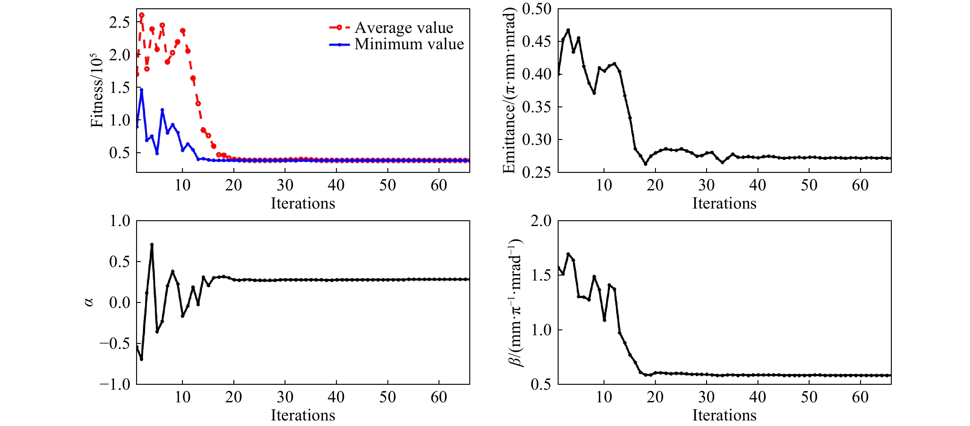
$ d_{i j} = SUM_{ij\_{\rm{sim}}}-SUM_{ij\_{\rm{exp}}} $ ,$ i $ indicates BPM number ($ i = 1 $ for BPM-5,$ i = 6 $ for BPM-10),$ n_{i} $ is the number of valid cases for the corresponding BPM. 30 sets of$ \{\varepsilon_{0}, \ \alpha_{0}, \ \beta_{0}\} $ are calculated as the first step, and the next step calculation is based on the fitness of the first step. With the number of steps increases, the minimum fitness decreases roughly. After about 60 iterations, all parameters become consistent, as shown in Fig. 7.After the PSO calculation, the consistent parameters are considered as the initial beam parameters at the exit of RFQ with the consideration of space charge effect.

Figure 7. (color online) PSO method for beam parameters calculation with space charge.
-
According to the definition of mismatch factor[5]
$M \!=\! \left[1+\frac{\varDelta+\sqrt{\varDelta(\varDelta+4)}}{2}\right]^{1 / 2}\!\!-1$ , where$\varDelta \!=\! \left(\alpha_{\exp}-\alpha_{\rm{sim}}\right)^{2}- $ $ \left(\beta_{\exp}-\beta_{\rm{sim}}\right)\cdot\left(\gamma_{\exp}-\gamma_{\rm{sim}}\right)$ , it is$ M = 0.478\,6 $ between the simulation results and experiment results with space charge, which is quite large and related analysis is needed.By replacing the initial beam parameters at the exit of RFQ by measured results in the experiment with the simulated parameters in Toutatis, no beam power loss is observed in downstream SC accelerating section in multiparticle tracking simulation in TraceWin (Fig. 8), which is in accordance with the fact that no obvious temperature rise in the SC section during the whole high power beam commissioning process. Since only longitudinal parameters are replaced, the beam envelope in the transverse plane stays at the same level, as shown in Fig. 9.
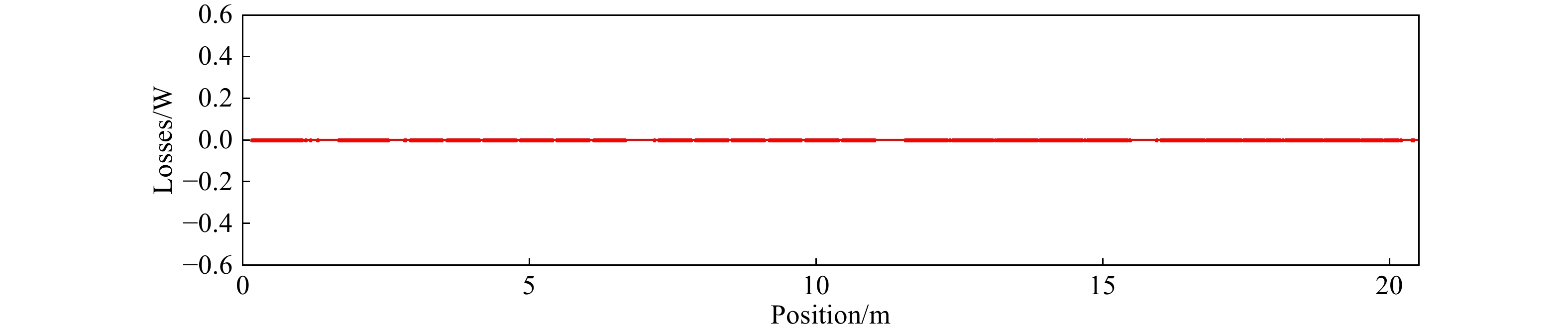
Figure 8. (color online) Power loss distribution. No power loss is observed along the linac in the simulation when replacing the initial longitudinal beam parameters at the exit of RFQ by measured results.
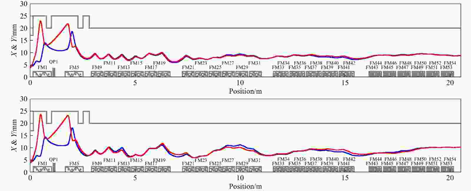
Figure 9. (color online) Transverse 5
$ \sigma $ envelope comparison. Blue line for$ X $ and red for$ Y $ . The top one is the simulation result, and the longitudinal input parameters for the bottom one come from the experiment results (Table 3).Beam envelope difference in the longitudinal plane is quite large, as shown in Fig. 10, but the RMS phase still stays almost within 5° during the former SC section, and the maximum value reaches about 20° in the last cryomodule. The density level distribution is compared for checking the details in Fig. 11, and it is within 200° for
$ 10^{-4} $ density probability for the maximum in the last cryomodule in multiparticle tracking simulation.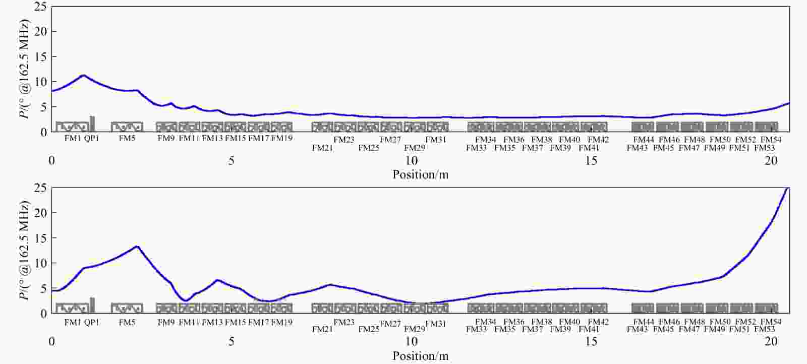
Figure 10. (color online) Longitudinal RMS phase comparison. As explained in Fig. 9, the top one is the simulation result, and the bottom one comes from the experiment results.

During the experiment, 6 BPMs located at different positions are used and the results from them could be considered as mutual verification. By the way, bunch shape monitors (BSMs) would be helpful for the verification in the future experiment. The simulation and experiment are based on the assumed ideal Gaussian distribution for the beam bunch in the longitudinal plane, which may be slightly different from the real situation. Local correction of the beam distribution will be considered for further study.
-
By adjusting the bunching voltage of the two bunchers at the MEBT of C-ADS accelerator, the longitudinal beam initial parameters at the exit of RFQ are measured by the SUM-signal of downstream 6 BPMs. Space charge effect is considered via the combination of the PSO method and TraceWin simulation. The measured emittance is close to the simulation results in Toutatis, but twiss parameters are quite different. Further study including BSM verification and beam distribution correction is under consideration.
Acknowledgments This work is supported by NSAF (Grant No. U1730122), and the Youth Innovation Promotion Association of Chinese Academy of Sciences under Grant No. 2018452.
-
摘要: 在C-ADS直线加速器样机中,为了描述束流相空间分布,需要精确测量束流在RFQ出口处的参数。束流横向信息已通过发射度重构测量获得,束流光学也得到了验证。采用了一种用BPM的SUM信号测量束流纵向参数的方法。在实验中,调节两台聚束器的聚束腔压并记录其下游BPM上的SUM信号。通过粒子群算法和TraceWin模拟相结合的方法,得到了考虑空间电荷效应的测量结果。测得的发射度与Toutatis中的模拟值相近。
-
关键词:
- longitudinal emittance measurement /
- twiss parameters /
- BPM /
- PSO
Abstract: To characterize the phase space distribution of the beam in C-ADS demo linac, beam parameters need to be measured with high accuracy at the exit of RFQ. Transverse information of the beam has been measured via the method of emittance reconstruction and the beam optics has been verified. A method has been adopted to measure beam longitudinal parameters by the SUM-signal of beam position monitors. The bunching voltage of the two bunchers and the SUM-signals in the downstream BPMs are recorded in the experiment. By combining the PSO(Particle Swarm Optimization) method with TraceWin simulation, the results are obtained with the consideration of space charge effect. The measured emittance is quite close to the simulated one in Toutatis.-
Key words:
- longitudinal emittance measurement /
- twiss parameters /
- BPM /
- PSO
-
Figure 3. (color online) Bunch length selection. Cases between the two layers ([27°, 122°]) are selected as valid data.
Figure 4. (color online) Simulated longitudinal bunch profile signals on different BPMs. (Pipe diameter and bunch length are different at the two locations).
Figure 6. (color online) SUM-current linearity verification for BPMs. (The square of the correlation coefficient for all the BPMs are beyond 0.9999).
Figure 7. (color online) PSO method for beam parameters calculation with space charge.
Figure 8. (color online) Power loss distribution. No power loss is observed along the linac in the simulation when replacing the initial longitudinal beam parameters at the exit of RFQ by measured results.
Figure 9. (color online) Transverse 5
$ \sigma $ envelope comparison. Blue line for$ X $ and red for$ Y $ . The top one is the simulation result, and the longitudinal input parameters for the bottom one come from the experiment results (Table 3).
Figure 10. (color online) Longitudinal RMS phase comparison. As explained in Fig. 9, the top one is the simulation result, and the bottom one comes from the experiment results.
Table 1. C-ADS demo linac parameters.
Parameters Value Unit Particle Proton — Energy 25 MeV Beam current 10 mA Duty factor 100 % Bunch frequency 162.5 MHz  下载: 导出CSV
Table 2. BPMs amplification coefficient. They are at almost the same level, which is in accordance with the BPMs' electronic characteristics.
BPM $ A_{0}\cdot \frac{I_{0}}{f_{0}}$ $ A_{0}$ BPM-5 1 001 453 28 965 BPM-6 885 538 25 612 BPM-7 820 576 23 734 BPM-8 807 598 23 358 BPM-9 819 124 23 692 BPM-10 817 776 23 653
下载: 导出CSV
Table 3. Beam longitudinal parameters at the exit of RFQ.
Parameters Simulation results
in Toutatis codeExperiment results
without space chargeExperiment results
with space chargeUnit $ {\varepsilon _{{\rm{Norm}},{\rm{RMS}}}}$ 0.297 8 0.543 2±0.025 8 0.271 5±0.024 6 $ {\rm{\pi }} \cdot {\rm{mm}} \cdot {\rm{mrad}}$ $ \alpha$ -0.254 5 0.559 9±0.002 4 0.285 0±0.005 7 — $ \beta$ 1.775 4 0.544 2±0.003 4 0.583 6±0.004 9 mm/$ ({\rm{\pi }} \cdot {\rm{mrad}})$
下载: 导出CSV
-
[1] LIU S H, WANG Z J, JIA H, et al. Nucl Instr and Meth A, 2017, 843: 11. [2] HUANG S, JIA H, NIU H, et al. Nucl Instr and Meth A, 2015, 799: 44. [3] SHISHLO A P. Novel Methods for Experimental Characterization of 3d Superconducting Linac Beam Dynamics[C/OL]// Proc North American Particle Accelerator Conf (NAPAC’13), Pasadena, CA, USA, Sep-Oct 2013.[2020-07-21]. https://accelconf.web.cern.ch/PAC-2013/papers/tuyb2.pdf. [4] REISER M. Theory and Design of Charged Particle Beams[M]. State of New Jersey: John Wiley&Sons, 2008: 74. [5] WANGLER T P. RF Linear Accelerators[M]. State of New Jersey: John Wiley&Sons, 2008: 285-286. [6] DUPERRIER R, FERDINAND R, LAGNIEL J, et al. [EB/OL]. [2020-07-21].https://accelconf.web.cern.ch/l00/papers/THB19.pdf. [7] URIOT D, PICHOFF N. Status of TraceWin Code[C/OL]// 6th International Particle Accelerator Conference, 2015. [2020-07-21]. http://accelconf.web.cern.ch/AccelConf/IPAC2015/papers/mopwa008.pdf. [8] SHISHLO A, ALEKSANDROV A. Longitudinal Diagnostics Methods and Limits for Hadron Linacs[C/OL]//5th International Beam Instrumentation Conference, 2017. [2020-07-21]. https://accelconf.web.cern.ch/ibic2016/papers/weal01.pdf. -

 点击查看大图

计量
- 文章访问数: 674
- HTML全文浏览量: 276
- PDF下载量: 63
- 被引次数: 0


 甘公网安备 62010202000723号